Jingjing Pan

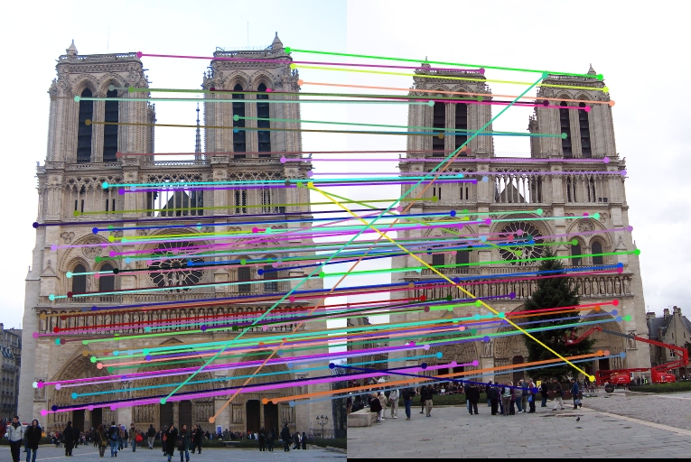
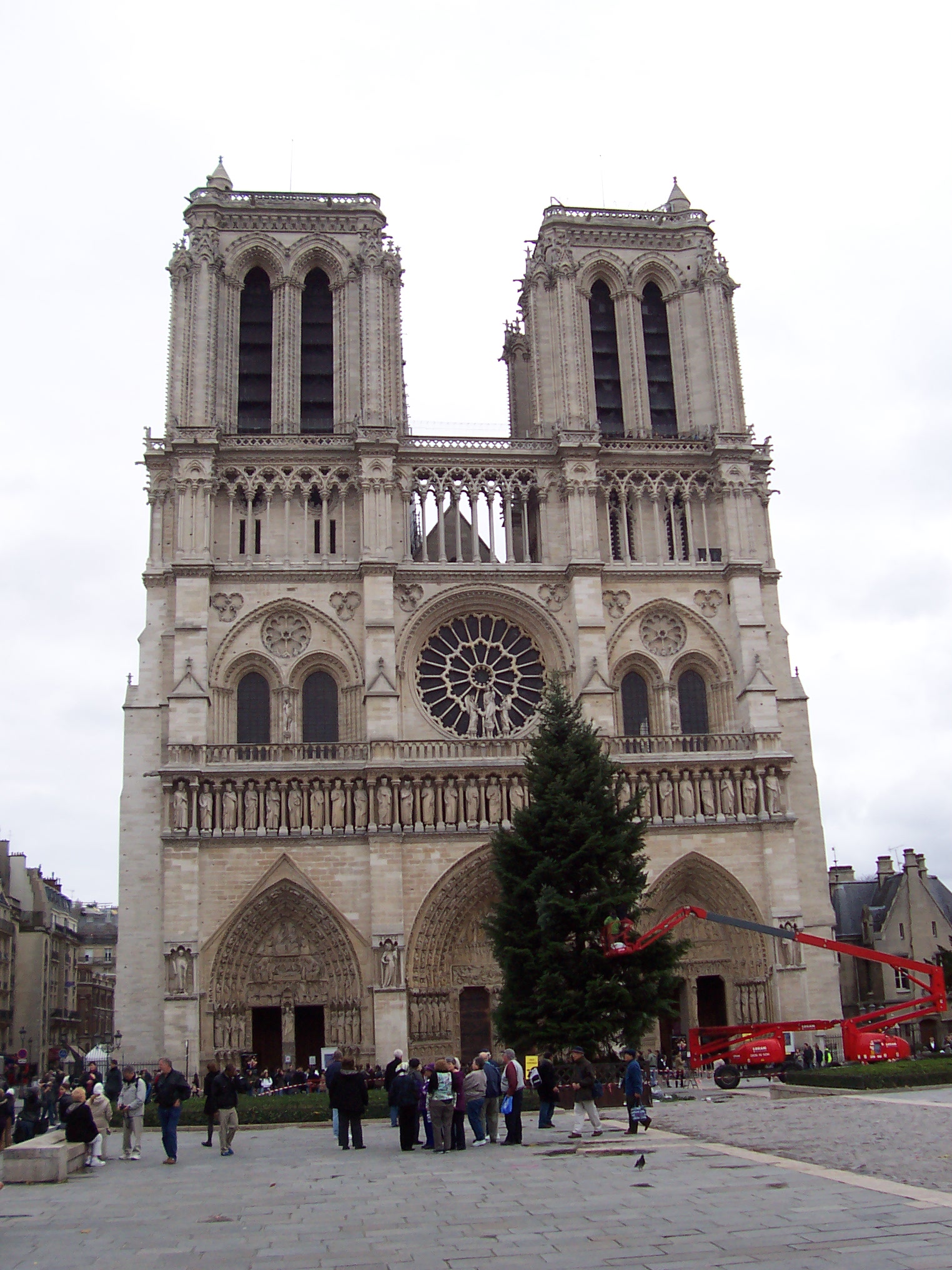
Local feature matching of two Notre Dame pictures

Algorithm pipeline

The three steps will be explained with Notre Dame example pictures and code below.

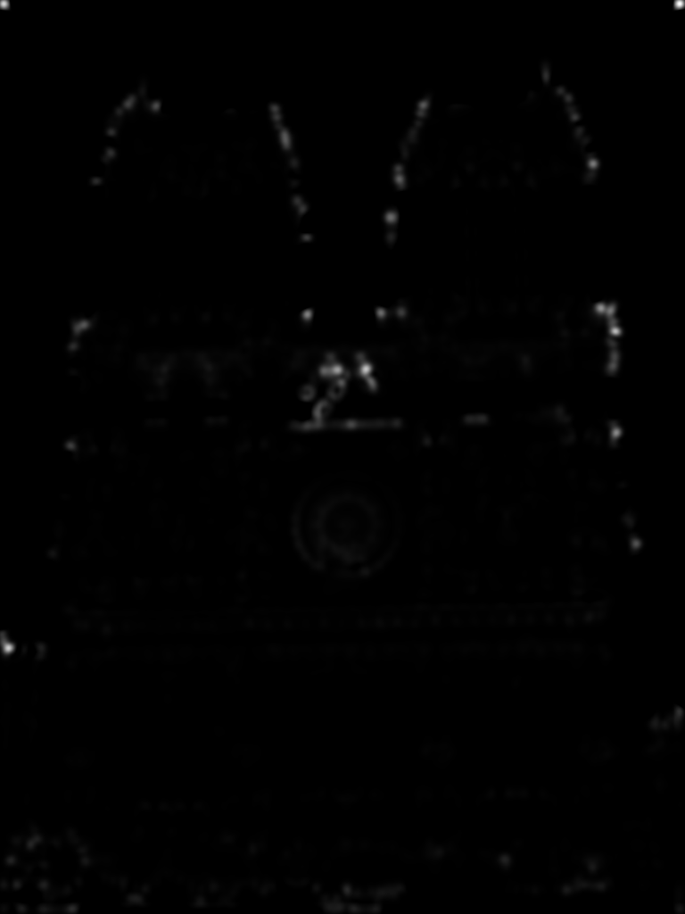
1. Interesting point detection

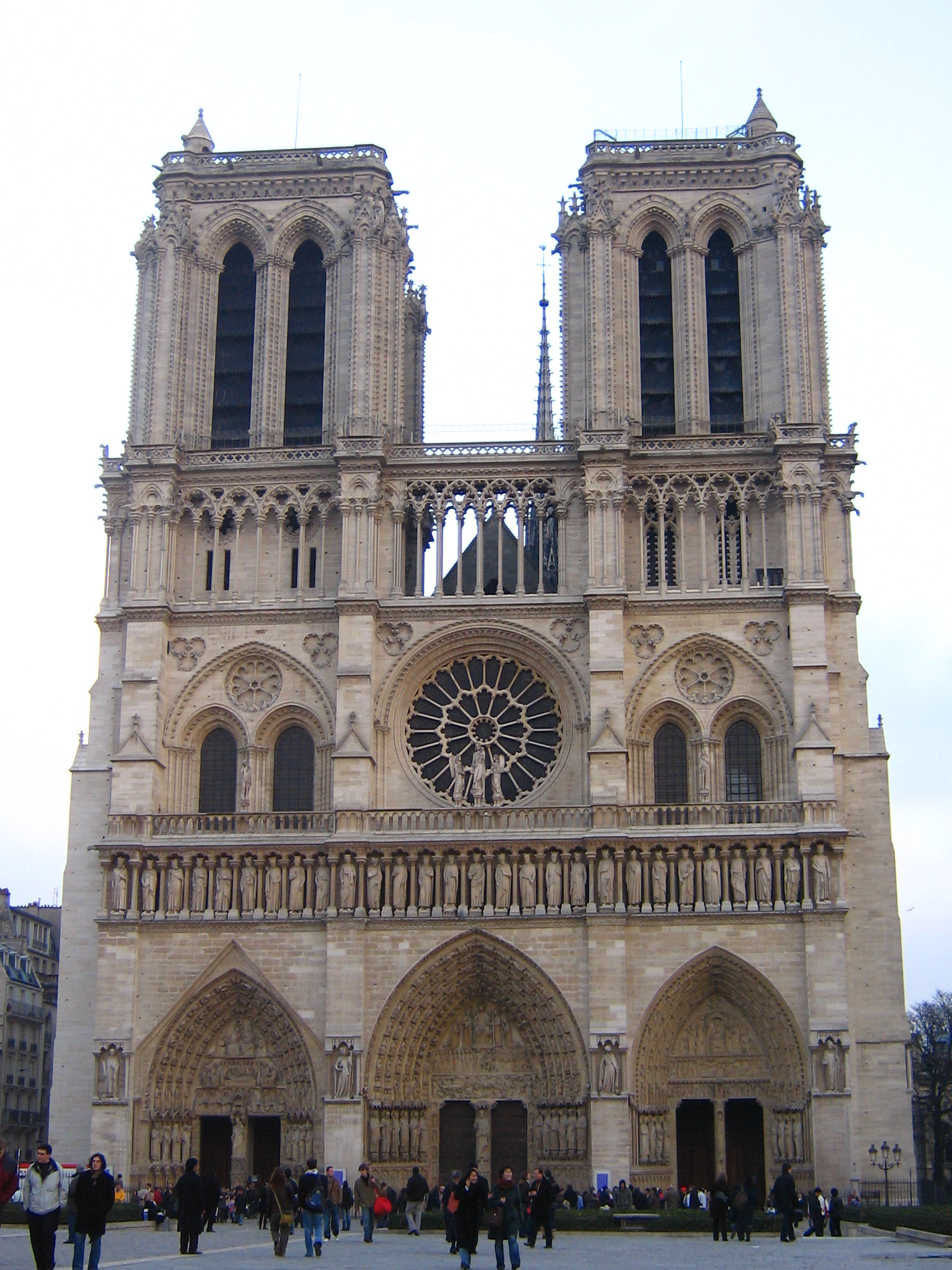
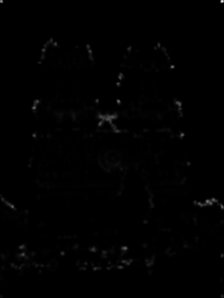
A main kind of interesting points is corners. Our algorithm uses Harris corner detector to produce around 1000 interesting points each from two input images of Notre Dame Cathedral taken from different angles and positions. (Visualization below shows cornerness after thresholding but before local non-maxima suppression in order to make interesting points more easy to see from screen.)

The cornerness M defined by Harris et al. (1998) can be implemented in MATLAB as:

[I_x,I_y] = imgradientxy(image);
Ix_2 = I_x.^2;
Iy_2 = I_y.^2;
Ixy = I_x.*I_y;

cut_freq = 5;
filter = fspecial('Gaussian', ceil(cut_freq*4), cut_freq);
g_Ix_2= imfilter(Ix_2, filter);
g_Iy_2= imfilter(Iy_2, filter);
g_Ixy= imfilter(Ixy, filter);

alpha = 0.04;
M = g_Ix_2.*g_Iy_2 - g_Ixy.^2 - alpha*(g_Ix_2+g_Iy_2).^2;

where cut_freq and alpha can be tuned for different image.

Since this actually gives us interesting "areas", we use a threshold to get rid of points with small cornerness, and then choose only points that have the local maxima in the sliding window surrounding it. Note that the later process can be easily implemented with 1) compute maxima map with function colfilt() with max() and then 2) compare maxima map with thresholded cornerness and supress (set to zero) pixels that do not have the same value in these two maps.

ths = 0.00001*max(M(:))
M_ths = zeros(size(M));
M_ths(M>ths) = M(M>ths);

sliding_width = 3;
M_max = colfilt(M_ths,[sliding_width sliding_width],'sliding',@max);
M_result = zeros(size(M_max));
idx = M_ths==M_max;
M_result(idx) = M_max(idx);

2. Interesting point detection

Second, we extract SIFT-like local feature from the 16x16 (feature_width by feature_width) square around each interesting point.

Specifically, for each interesting point, we first extract the 16x16 patch around it and compute gradient magnitude and orientation at each pixel:

patch = image(r_start:r_start+feature_width-1, c_start:c_start+feature_width-1);
[mag, ori] = imgradient(image);

Then we devide each patch into 4x4 grid of cells. Each cell has 4x4 pixels. We find gradient magnitude and orientation for each cell and let the magnitutes contribute to their corresponding orientation bins, which gives us 8 voting results for each cell. In this way, we get 16 cells * 8 bins = 128 numbers for each interesting point.

ori_cell = ori(1+(k-1)*cell_width:k*cell_width, 1+(j-1)*cell_width:j*cell_width);
ori_cell = ori_cell(:);
mag_cell = mag(1+(k-1)*cell_width:k*cell_width, 1+(j-1)*cell_width:j*cell_width);
mag_cell = mag_cell(:);
votes = zeros(1,8);
for m=1:length(ori_cell)
	ori_this = ori_cell(m);
	mag_this = mag_cell(m);
	for n=1:8
		lower_bound = -180+45*(n-1);
		if ori_this >= lower_bound && ori_this < lower_bound+45
			votes(n) = votes(n) + mag_this;
			break
		end
	end
end
% votes
cell_idx = (k-1)*4+j;
feat((cell_idx-1)*8+1:cell_idx*8) = votes;
% unit-length normalization:
feat = feat./sqrt(sum(feat.^2));

With this implementation, We obtained 80.0% matching accuracy in Notra Dame pair. However, it is worth mentioning that using raw intensity from the 16x16=256 pixels around it also gives a 74% accuracy in this case.

3. Matching features

We find point pair from image 1 and image 2 so that their features have the least L2 distance, and we can say these two points are likely to be the same point on the object instance. In our pipeline, for each interesting point in image 1, we look for the interesting point in image 2 that has the least L2 distance of feature with it.

for i=1:num_features
	feat1 = features1(i, :);
	feat1_rep = repmat(feat1, num_features, 1);
	l2_dist = sqrt(sum((features2 - feat1_rep).^2, 2));
	...
	...
end

Moreover, to make the matching more accurate, we can define confidence for each matching like below. The analogy is that the similarity of best matching points should be much smaller than and very distinctive from that of the second best matching for a confident matching.

[dist_sorted, dist_idx] = sort(l2_dist, 'ascend');
dist_nn1 = dist_sorted(1);
idx_nn1 = dist_idx(1);
dist_nn2 = dist_sorted(2);
idx_nn2 = dist_idx(2);

% compute distance ratio for nn1 and nn2
confidences(i,1) = 1 - dist_nn1/dist_nn2; 

Result local feature matching from some examples

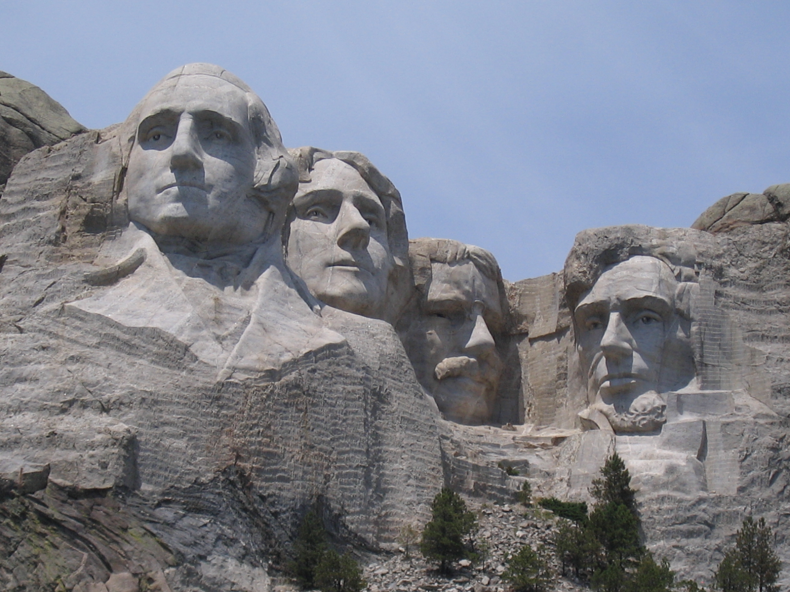
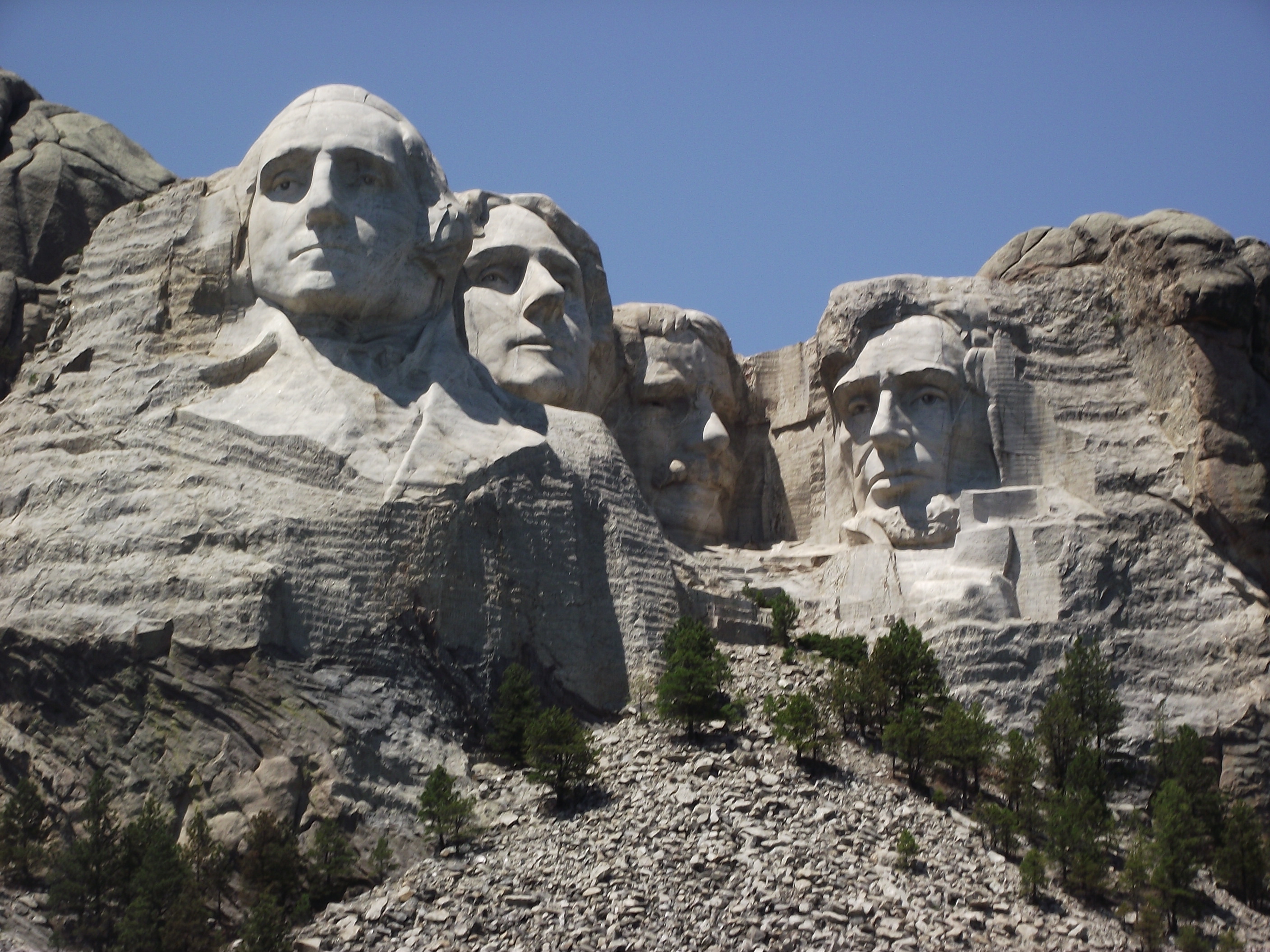
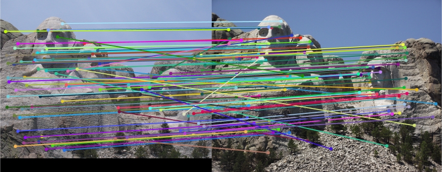
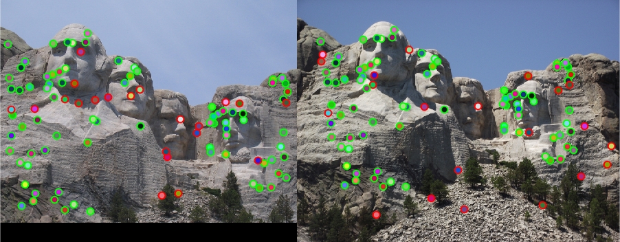
Mount Rushmore

With the same parameters tuned for Notre Dame pair, Mount Rushmore got 79% accuracy in the top 100 matchings, which is not bad. So I did not tune parameter for this pair.

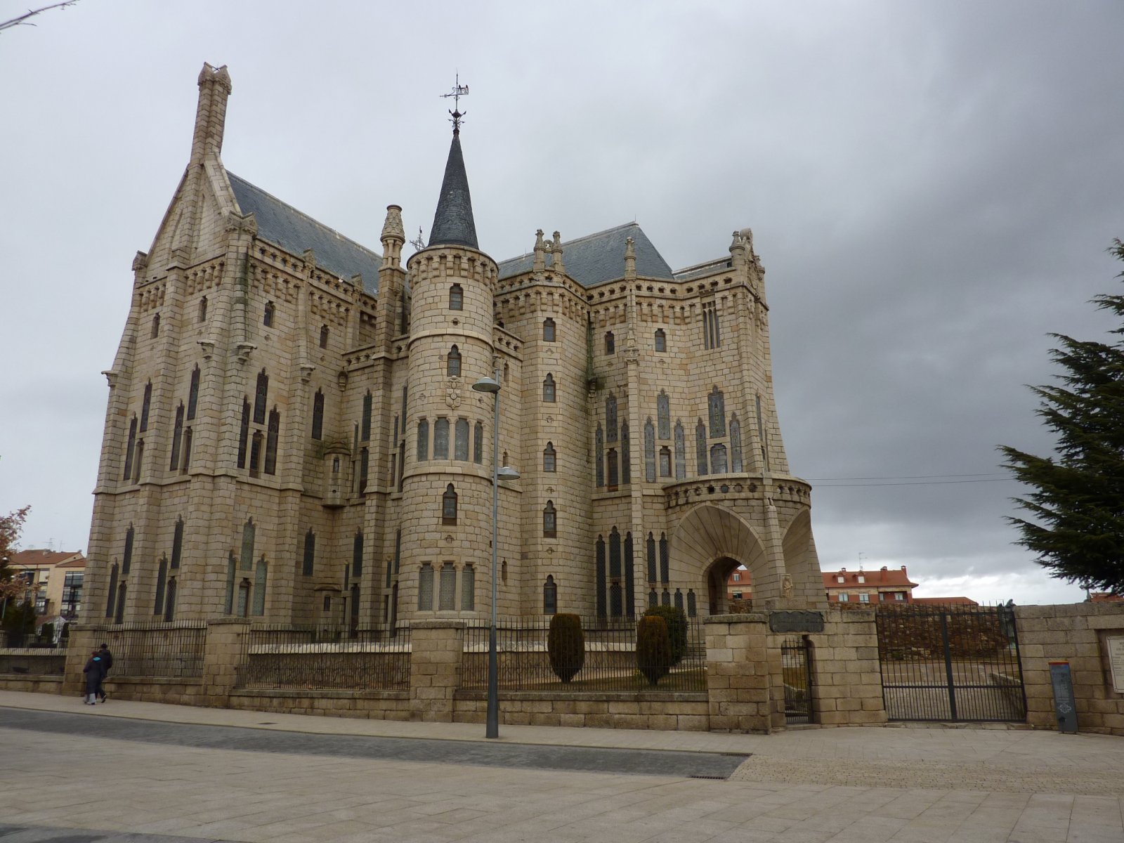
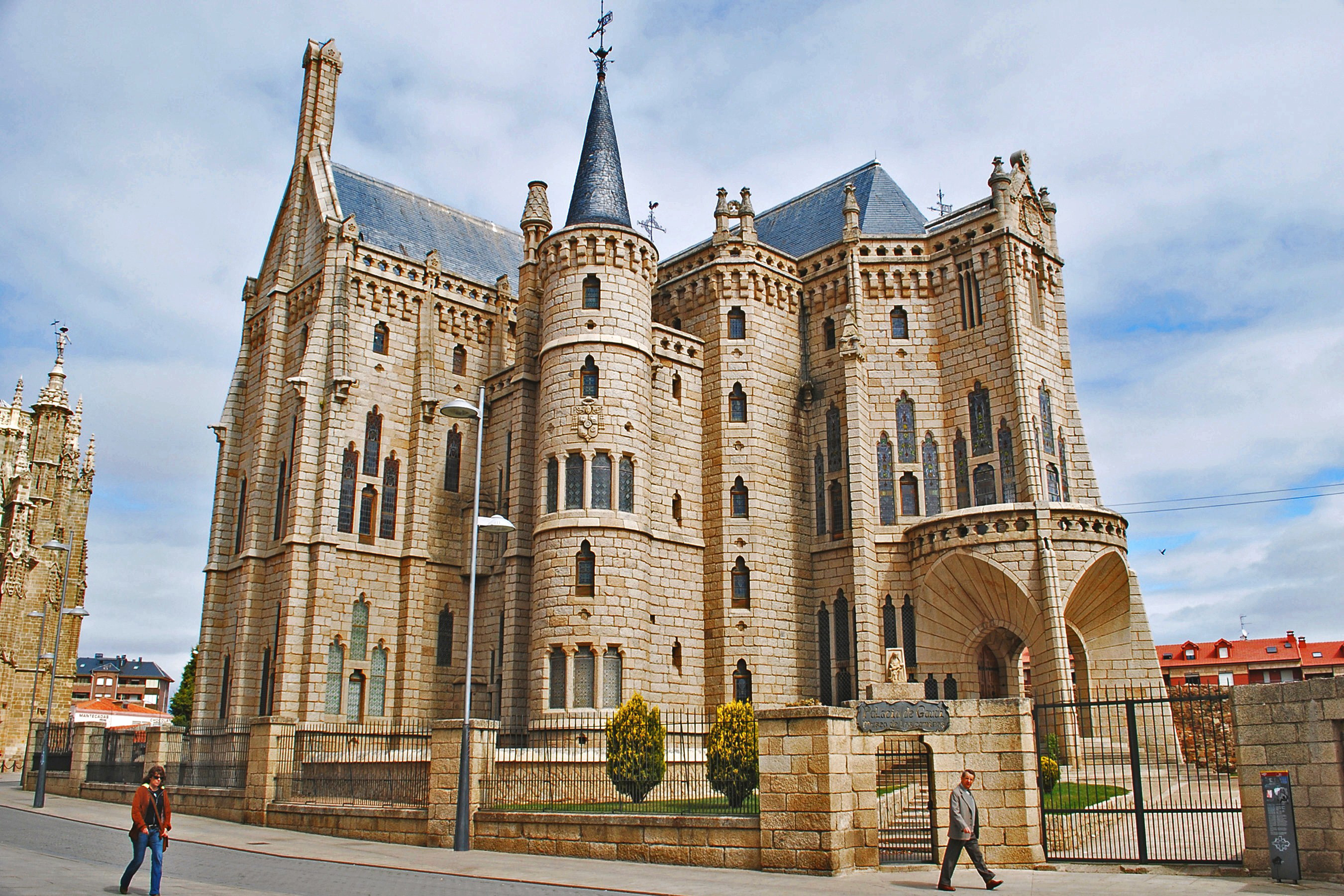
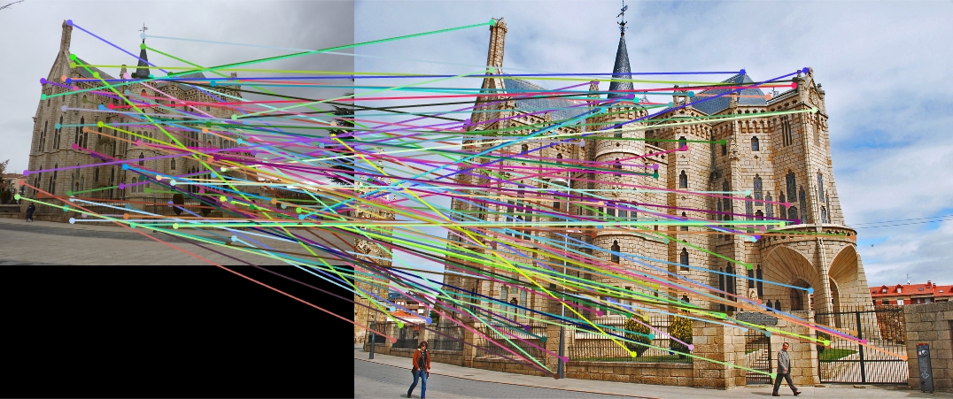
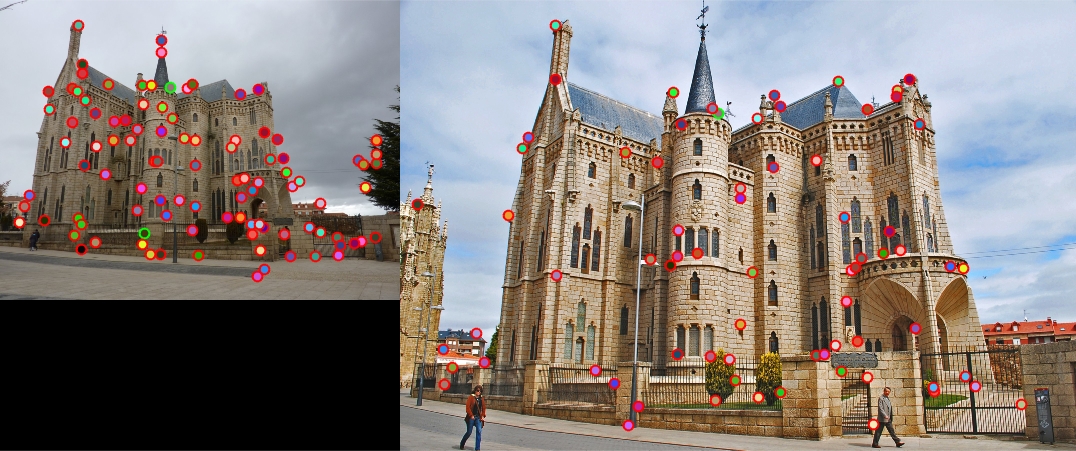
Episcopal Gaudi

With the same parameters tuned for Notre Dame pair, Episcopal Gaudi can only get 2% accuracy, which is not a desired result. After parameter tuning, so far I can only get 3% accuracy. The reason could be the over-simplification of our pipeline (using Harris cornerness to present importance of points, using simplified version of SIFT feature, ignorance of variance in scales, nearest neighbor matching, etc. This pair has a much more obvious angle shift than the first two pairs, which also increases the complexity of this problem.

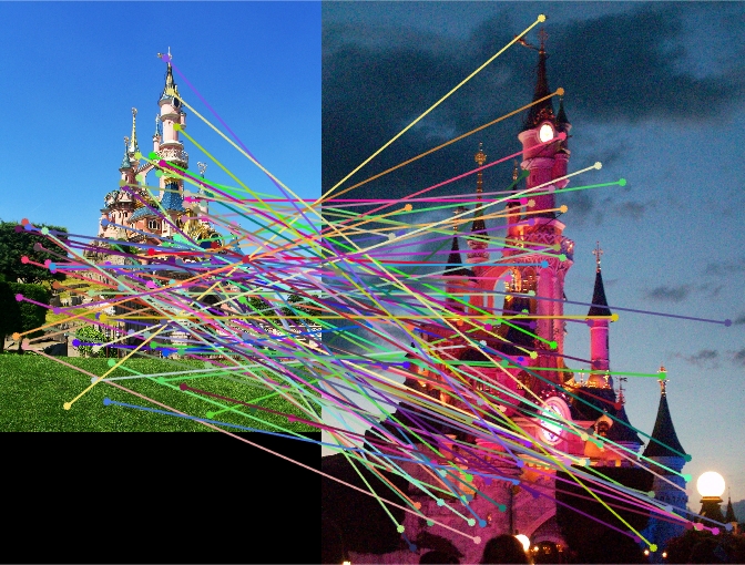
Sleeping Beauty Castle in Paris

One interesting case in extra_data examples is the pictures taken under different lighting condition. It is obvious that the interesting points detected can be more different positions on the instance and the feature extracted could be very different between the same instance position, which can both bring down the matching accuracy.

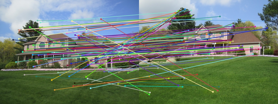
House

However, this simplified algorithm still works well with image pairs that do not have much scale, lighting and angle variation.