James Jonghan Park

get_interest_points.m
alpha = 0.06; % alpha value used for Harris equation.
sigma = 1; % Sigma used for Gaussian filter after image derivatives.
multSigma = 1; % Sigma used for Gaussian filter after square of derivatives.
threshold = 0.01; % Threshold used for creating a binary image in bwconncomp

match_features.m
threshold = .66; % Maximum tolerable distance for nearest neighbor
dimensions = 100; % Dimenions to keep for dimensionality reduction (PCA)

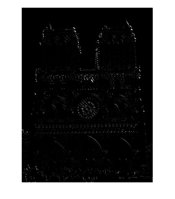
Interest point detection

In order to begin our local feature matching, it is good to find interest points or distinctive points for feature matching. We will use a popular algorithm called Harris corner detector.

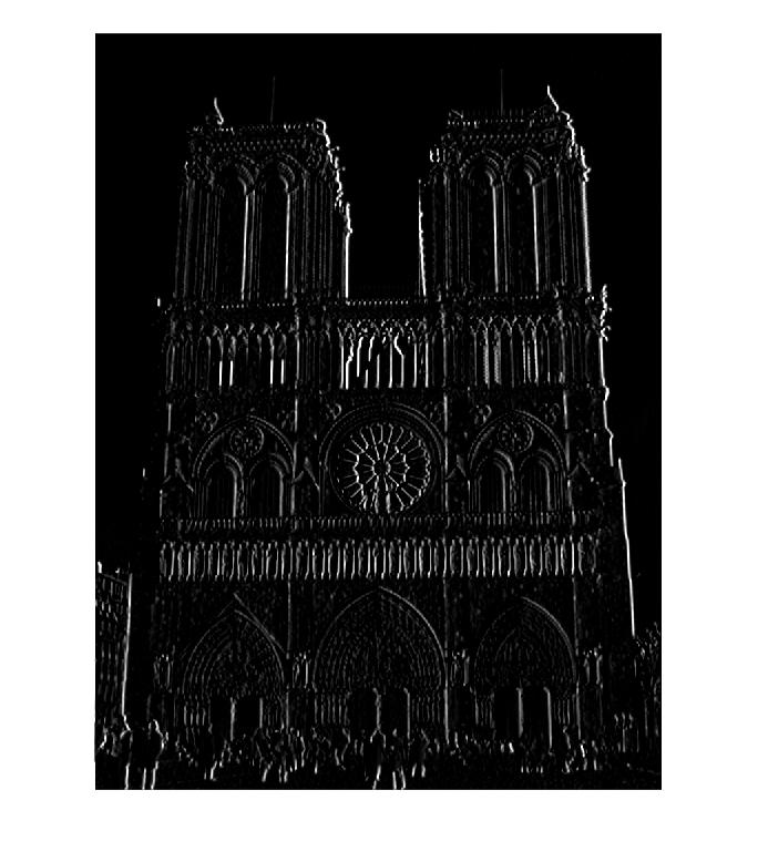
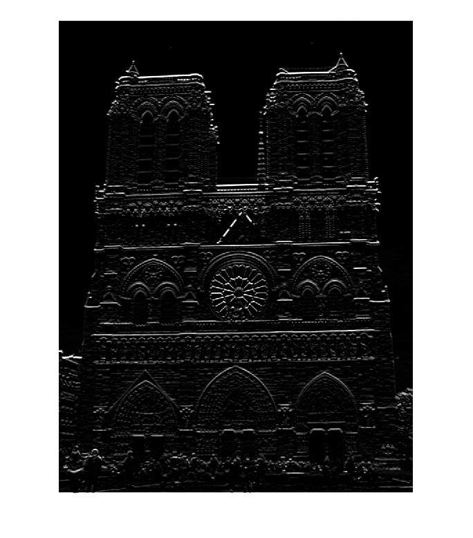
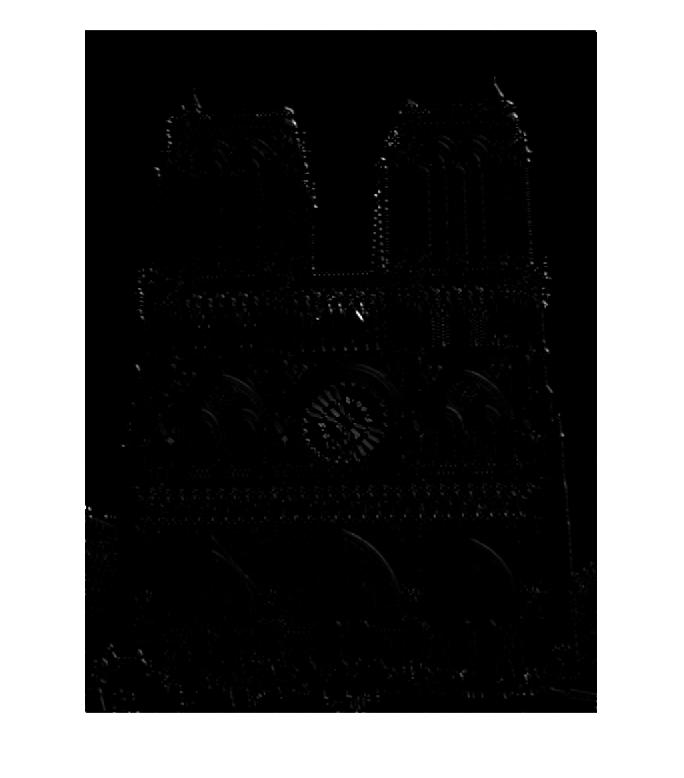
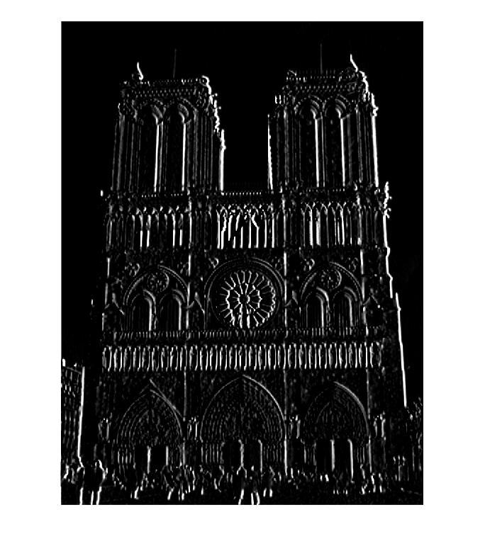
We blur the image and take the image derivatives using Sobel filter. Then take the square of derivatives and blur the image again using Gaussian filter. Sobel filter is mostly used for edge detection, where an image is filtered to show edges.
Finally, use those values for Harris cornerness function:
Left to right: Ix, Iy, Ixy, Ix^2, image computed on cornerness function.
We suppress several points here.
1. Boundary points
This helps to prevent index out of bounds exception when obtaining features for each interest points.
2. Non-maximum points
We want to keep local maxima points as our interest points. I used BWCONNCOMP to find connected components in thresholded binary image, and took the maximum value within each component. The remaining points are selected as interest points.

Local feature description

Each interest points should be assigned with a descriptor so that they can be compared and matched across different sets of images. I now introduce a SIFT-like implementation.
For each set of interest points, we obtain a square patch of image around the interest point, where width is defined by feature_width. The square of patch will not be exactly centered around the interest points, because SIFT utilizes an even feature_width. We apply each patch with a gradient, where we will obtain magnitudes and angles to construct our descriptor. We subdivide our patch and create a histogram of angles, where the values of each entry will be the sum of magnitudes corresponding to angle bins. We combine these histograms to create a feature. The features are normalized, the values above threshold are clamped to the value of threshold, and renormalized.

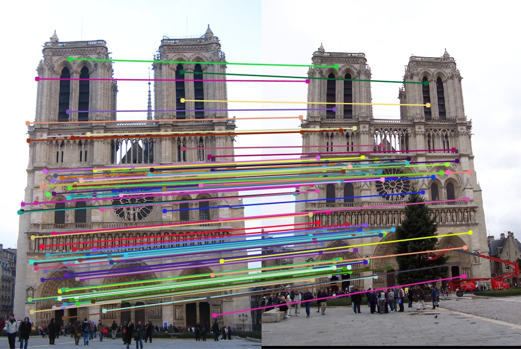
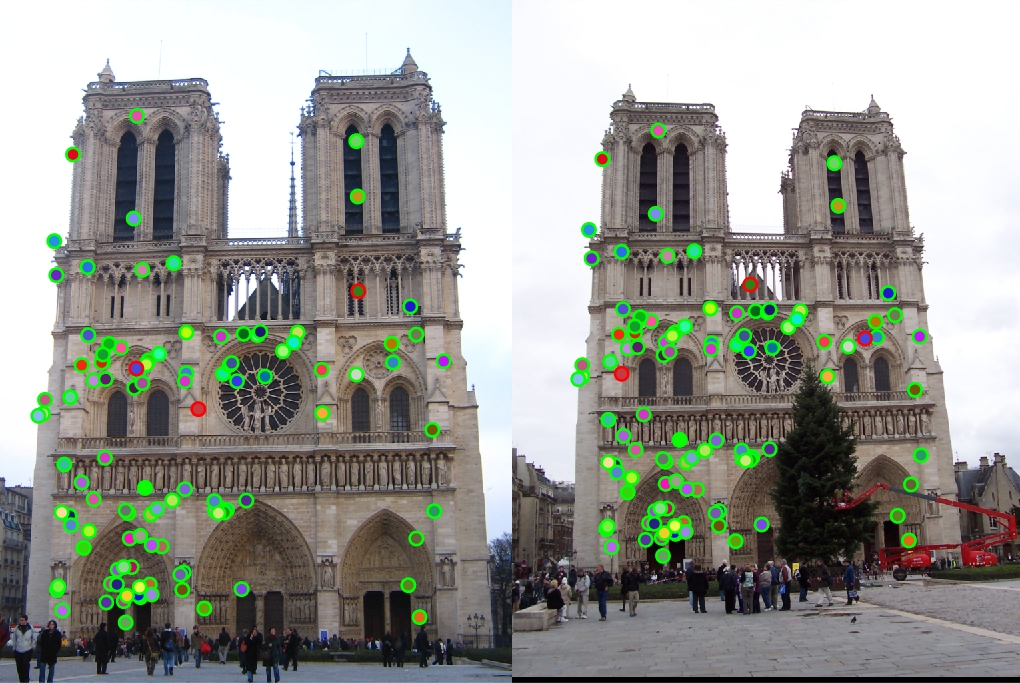
Feature matching

We are ready to match our interest points across different sets of images using our features. For this process, we use our constructed features and apply nearest neighbor distance ratio test. To do this, we retrieve two nearest neighbors using knnsearch with kdtree. Each of two nearest neighbors are divided for ratio test, and we also get rid of ones that exceed our threshold. Not always, but it's likely that closer resembling neighbors are correct matches. In this code, I also implement PCA, which is used for dimensionality reduction. This reduces our dimensions, allowing to reduce the number of costly calculations (if calculations are expensive). We reduce the number of dimensions by maximizing variance. Sometimes dimensionality reduction increases accuracy if the input parameter is very noisy; however, generally it reduces accuracy for performance. In our case, we maintain high accuracy rate with Notre Dame.

Results

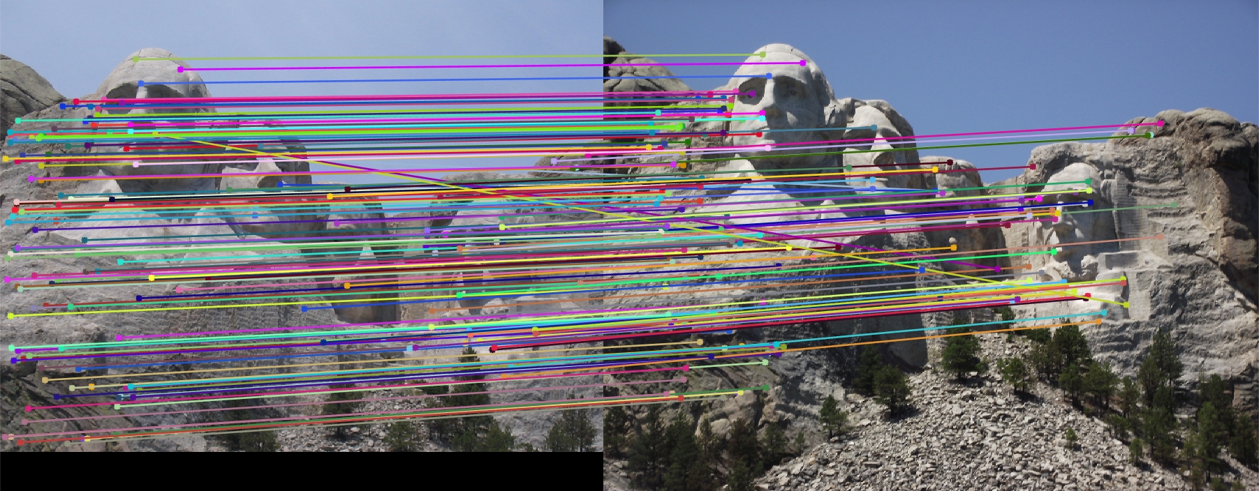
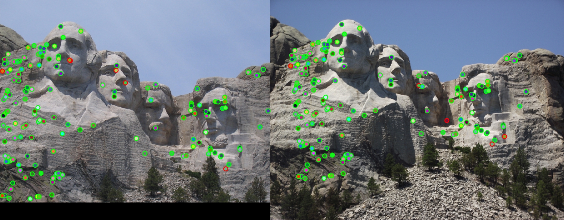
For images that have easy to detect corners with similar viewing rotations and scales, we have high performance.
For Notre Dame, we get: 106 total good matches, 3 total bad matches. 0.97% accuracy.
For Mount Rushmore, we get: 154 total good matches, 6 total bad matches. 0.96% accuracy.

Sadly for images that have conflicting scale + rotation, my algorithm detected zero matches. My code is not optimized for scale and rotation invariance.