Project 2: Local Feature Matching
This project is an implementation of feature matching across images. To accomplish this, the project is broken into three parts:
- Feature Detection
- Feature Discription
- Feature Matching
1. The Algorithm: Feature Detection
In order to implement the Feature Detection, I used a Harris detector algorithm. The algorithm can be broken into the following steps:
| 1.1 Compute horizontal and vertical derivatives of images | To accomplish this, I used MATLAB's built in function "imgradientxy(I)" which is equvalent to applting the vertical and horizontal sobel filter to the image. The derivatives are shown to the right. | 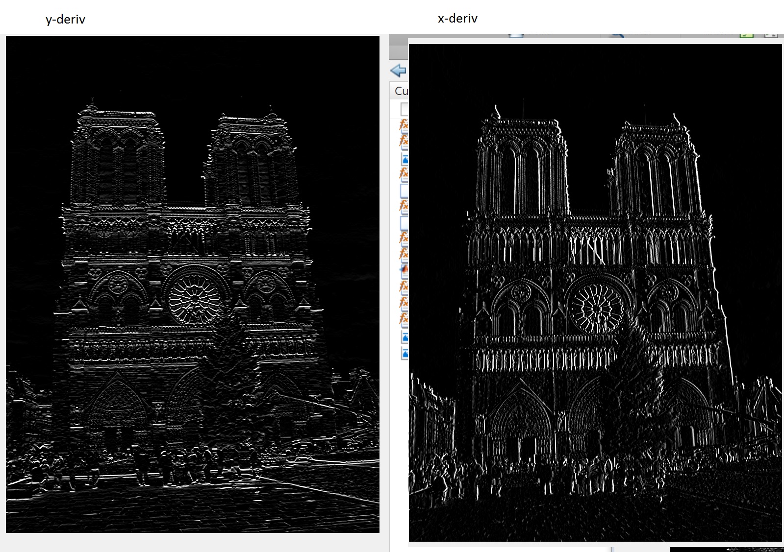 |
| 1.2 Compute (dy)^2, (dx)^2, and dy(dx) | To accomplish this, I simply took the horizontal and vertical derivatives and did element-wise multiplication on them | |
| 1.3 Convolve image with larger Gaussian | To accomplish this, I created a 7x7 gaussian filter with sigma = 1. Then, I applied it to each of the values computed in 1.2 | |
| 1.4 Compute Corner Response | I created a matrix for the corner response at each pixel by following the corner response function. In this case, the determinant of M would be (dy)^2(dx)^2 - (dy(dx))^2, and the trace would be (dy)^2, (dx)^2. I'm using an alpha value of .6. The corner response function is to the right. |  |
| 1.5 Find local maxima above a trheshold | Here, I first suppressed all the values below my chosen threshold of .005 to be 0. Afterwards, I used MATLAB's function bwconncomp() to find connected pixels. I then only reported the maximum xy of each area of connected pixel. Additionally, I suppressed all features along a border of size feature_width/2 so that every reported feature can use the entire area around it when making its descriptor. |
2. The Algorithm: Feature Discription
During the process of this project I attempted 3 different types of fearure descriptor algorithms
| 16x16 Image patch around the feature | This feature descriptor simply cuts out a 16x16 patch from the image around the feature and uses that patch as the descriptor. For the top 100 matches, I was able to achieve a 75% accuracy. The matching is shown on the right. | 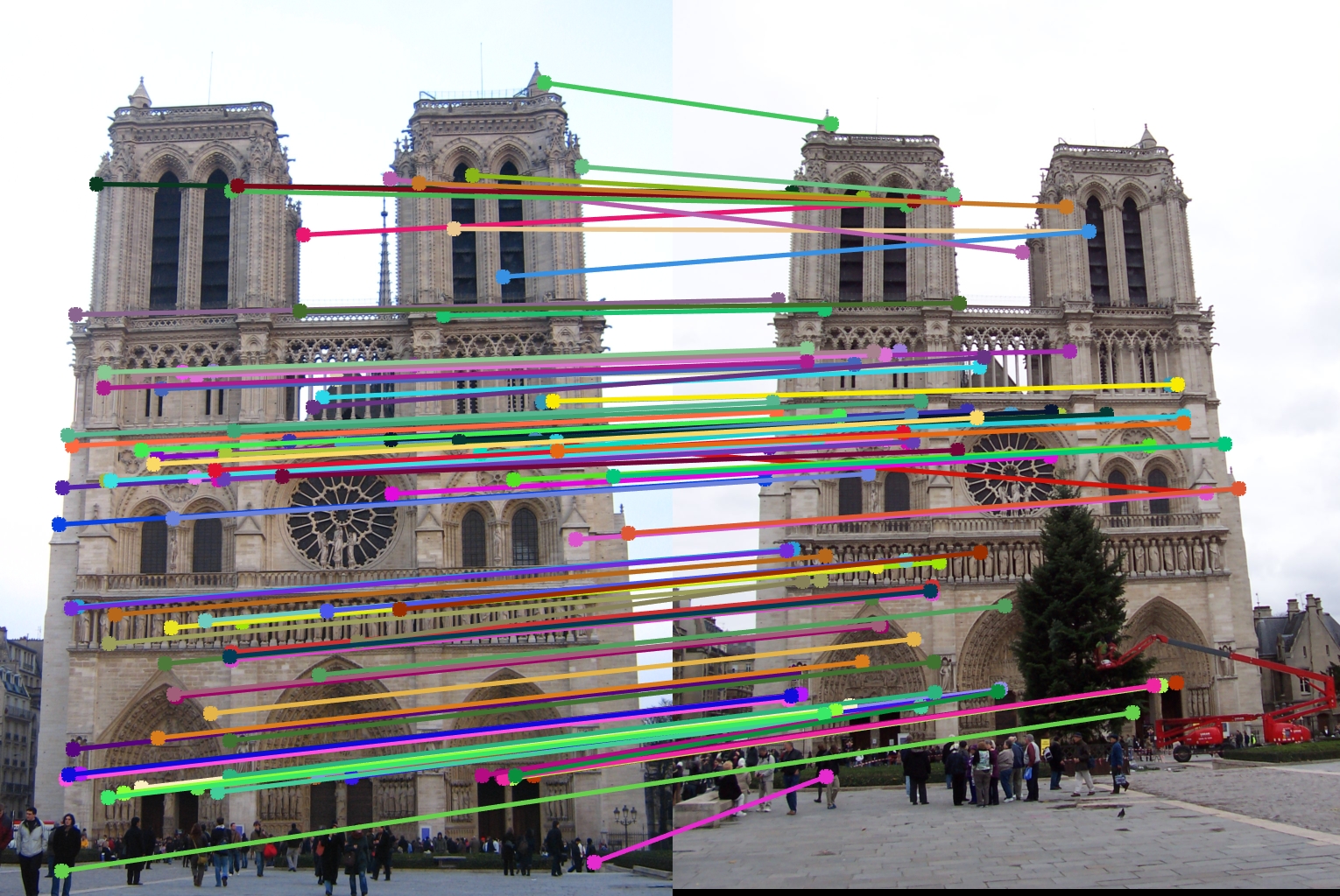 |
| SIFT-Like descriptor using rotated sobel filters to get gradients | This descriptor takes images patches around each feature and filters them along 8 directions using rotated sobel filters. Then, it takes divices the patch into 4x4 cells and for each cell, and for each direction, sums the gradient. The descriptor was normalized, thresholded at .2, and normailzed again. The final descriptor is then raised to the power of .5. I was able to achieve 82% accuracy for the top 100 matches. The matching is shown on the right. | 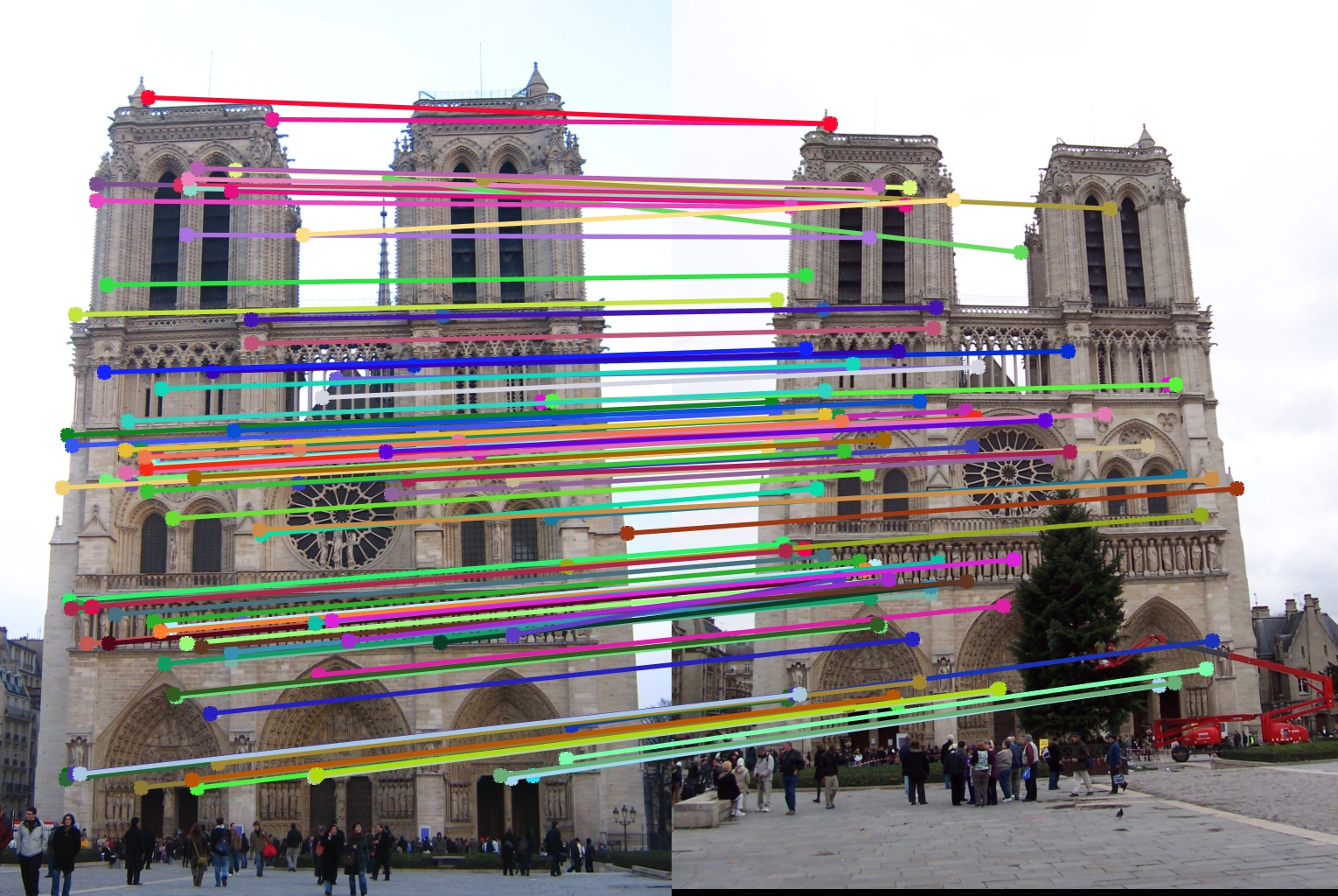 |
| SIFT-Like descriptor using trig to get gradients | This descriptor is the one that is closest to SIFT. It first takes a gradient of the image. Then, it looks at a patch around each feature. These patches are then divided further into 4x4 cells. For every pixel in the cell, the gradient is projected onto the nearst two directions of 8 standard directions. The projections are then used as the descriptor. The final descriptor is then raised to the power of .5. The descriptor was normalized, thresholded at .2, and normailzed again. I was able to achieve an 89% accuracy with this descriptor for the top 100 matches. The matchings are shown on the right. Projecting into more than 2 directions only resulted in a loss of accuracy. | 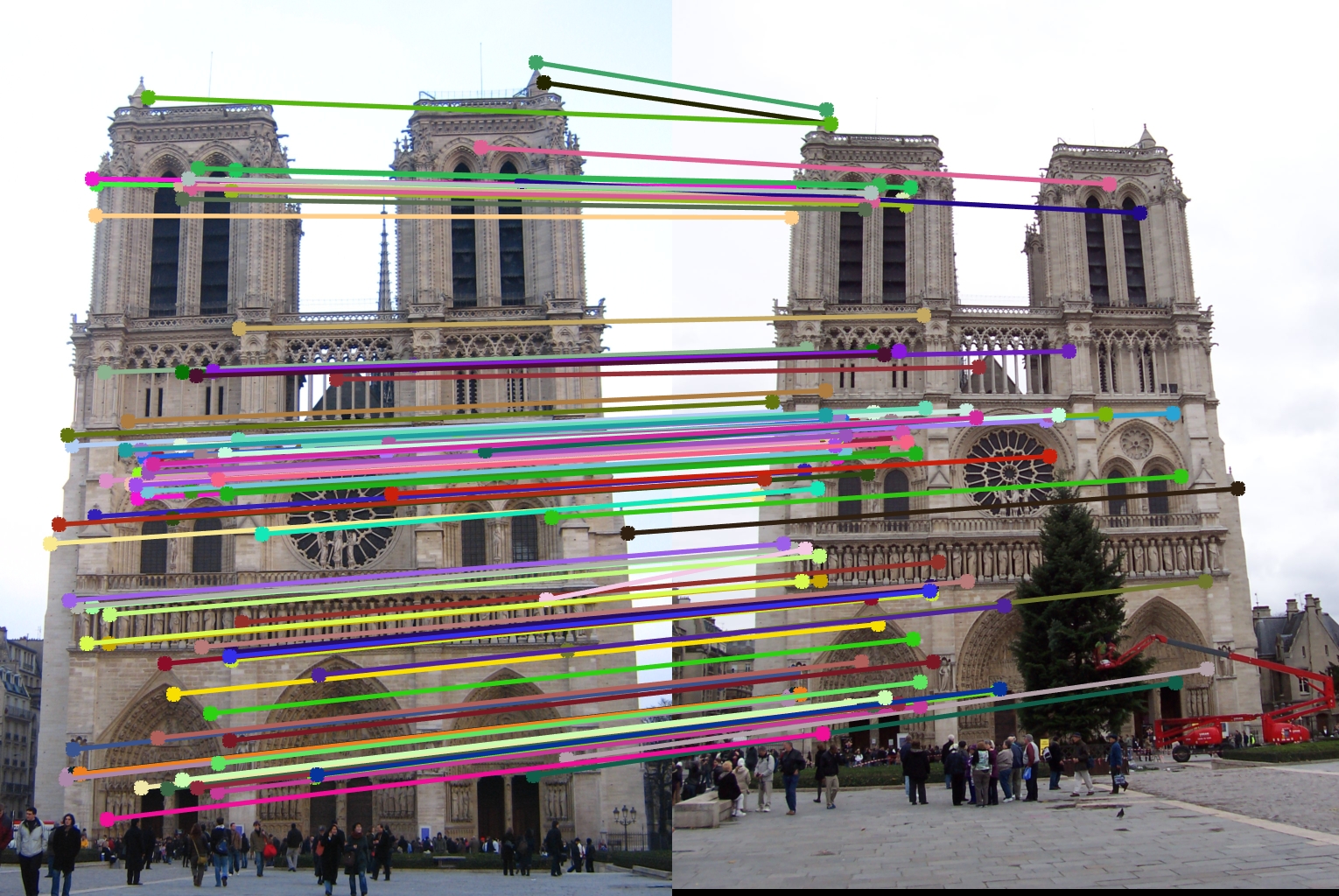 |
3. The Algorithm: Feature Matching
The feature matching algorithm uses euclidean distances to find the distances between tresholds. For each feature point in the first image, the matching algorithm will find the nearest match in the second distance. Next, the matching algorithm uses the ratio test to determine confidence of each match. As long as eatch match passes the ratio test with a certain threshold, then it can be considered a match. The matches are then sorted in order of confidence.
I expperimented with the matching threshold with the notre dame image set. As the threshold increases, the accuracy should increase, but there will be less matches. For example, using .4 instead of .25 as the threshold increased the accuracy from 89% to 96%, but there are only 28 total matches. A threshold of .25 was giving me the best result with at least 100 matches after testing several values of the parameter.
4. Results
This feature matching process was tested on 3 image sets. Over all three sets, there were no noticible issues in run-time or memoory usage. The algorithm never took my more than 15 seconds to run. For all of the image sets, I used the SIFT-Like descriptor using trig to get gradients as it seemed to give me the most accurage matches.
| Image Set | Accuracy for top 100 features | Matching Threshold | Eval |
| Notre Dame | 89% | .25 | 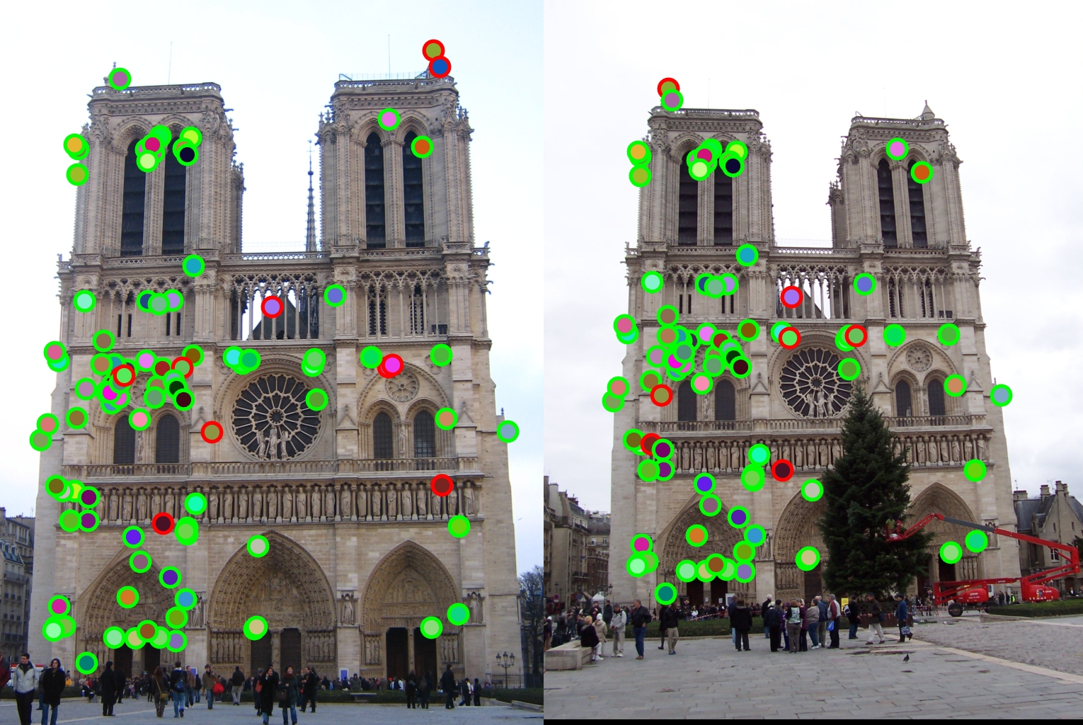 |
| Mount Rushmore/td> | 98% | .25 | 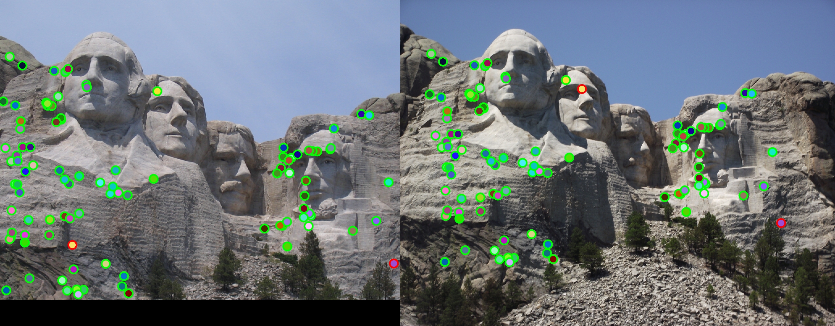 |
| The next image was unable to achieve 100 matches with the matching threshold of .25, so I lowered it to .05 | |||
| Episcopal Gaudi | 7% | .05 | 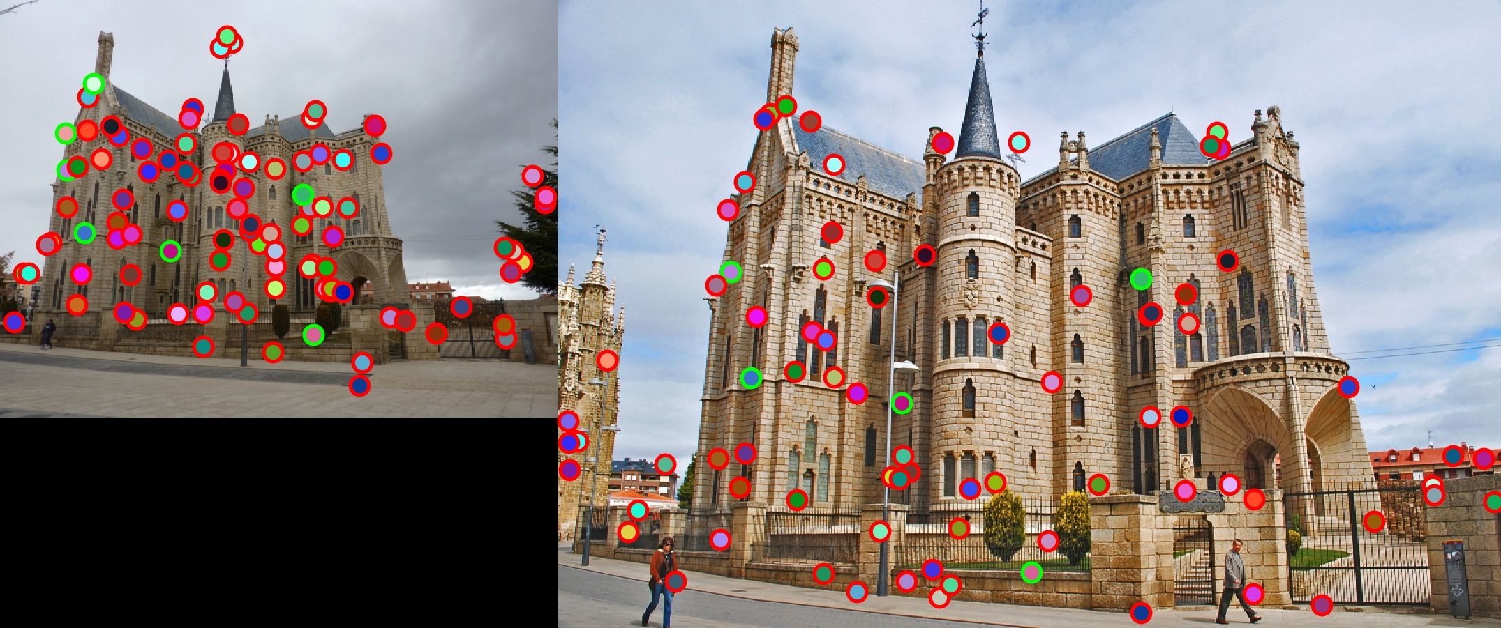 |
The combination of a Harris feature detector and a SIFT-like feature descriptor can produce vary good results as seen in the Mount Rushmore and NotreDame image sets. However, it appears to have issues wiith the Episcopal Gaudi image set. This is almost certainly due to the different scale of the images; I didn't do any work to make the feature descriptors scale-invariant nor rotationally-invariant.