Computer Vision Project

In this project, we are going to implement the local feature matching algorithm based on Szeliski chapter 4.1. I use Harris Corner Detector for interest points detection, simplifies SIFT feature as feature descriptor and "nearest neighbor distance ratio test" to order the feature matching. Based on my implementation and some parameter-tuning, if I only evaluate the most confident 100 matches on the Notre Name pair, I can achieve 97% accuracy.

Algorithm

Feature Matching (match_features.m)

For each interest point A in Image 1, we will seach for its nearest neighbor B and sencond nearest neighbor C among all interest points in Image2. We will treat (A,B) as possible interest points matching pair. In addition, we apply the nearest neighbor distance ratio (equation shown in the Fig 2) here. We define 1/NNDR as the confidence for the particular pair.

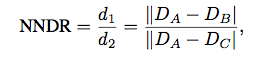
Fig 2. Equation for nearest neighbor distance ratio.

SIFT Feature Extraction (get_features.m)

For each interest point, I will calculate its features based on the feature_width*feature_width region around it. Firstly, I will divide the square region into a 4x4 grid of cells, each feature_width/4. We need to generate a 1*8 feature vector for each cell. Using imgradient() provided by Matlab, we can easily calculate the direction and magnitude of gradient for each pixel. We accumulate the magnitude according to 8 different standart direction (Fig 3) and the accumulation values will be features for that particular call. Note: In my implementation, I will add the magnitude to two nearest directions instead of one.

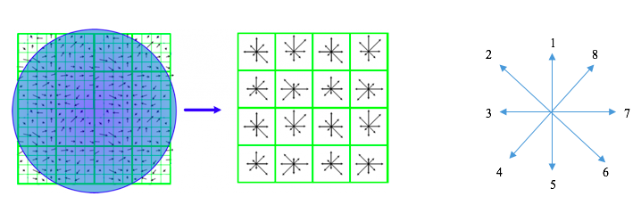
Fig 3. Illustration of spatial of my SIFT and the 8 standard directions.


%Generating the 1*8 feature vector for each cell
%Looping in the cell and use temp_feature to store the feature vector
%The magnitude of each gradient will contribute to the nearest two standard directions
temp_feature=zeros(1,8);
for xx=xi:xi+feature_width/4-1
    for yy=yi:yi+feature_width/4-1
        temp_feature(Gdir_range(yy,xx))=temp_feature(Gdir_range(yy,xx))  ...
        +Gmag(yy,xx)*cosd(Gdir(yy,xx)-45*(Gdir_range(yy,xx)-1)+180);
        temp_feature(mod(Gdir_range(yy,xx),8)+1)=temp_feature(mod(Gdir_range(yy,xx),8)+1) ...
        +Gmag(yy,xx)*cosd(-180+45*Gdir_range(yy,xx)-Gdir(yy,xx));
    end
end

Interest Point Detection (get_interest_points.m)

To detect the interest points, I make use of the Corner Response Equation (Figure 4). Higher response value means that the points are more likely to be corner. And then I will select points which have local maximal value in every 5*5 area of R as the interest points.

Fig 4. Corner Response Equation.

Extra Credit

Try detecting keypoints at multiple scales

For the Notre Dame image pair, I try different scale. When the scale become larger, the number of keypoints I can detect will be larger and thus the program will run for longer time. But image in larger scale will contain more details, it sometimes will help the pipeline to get higher accuracy. So there is a trade-off. From Fig 5, we can figure out that the accuracy for this image pair almost become largest when scale goes to 0.5.

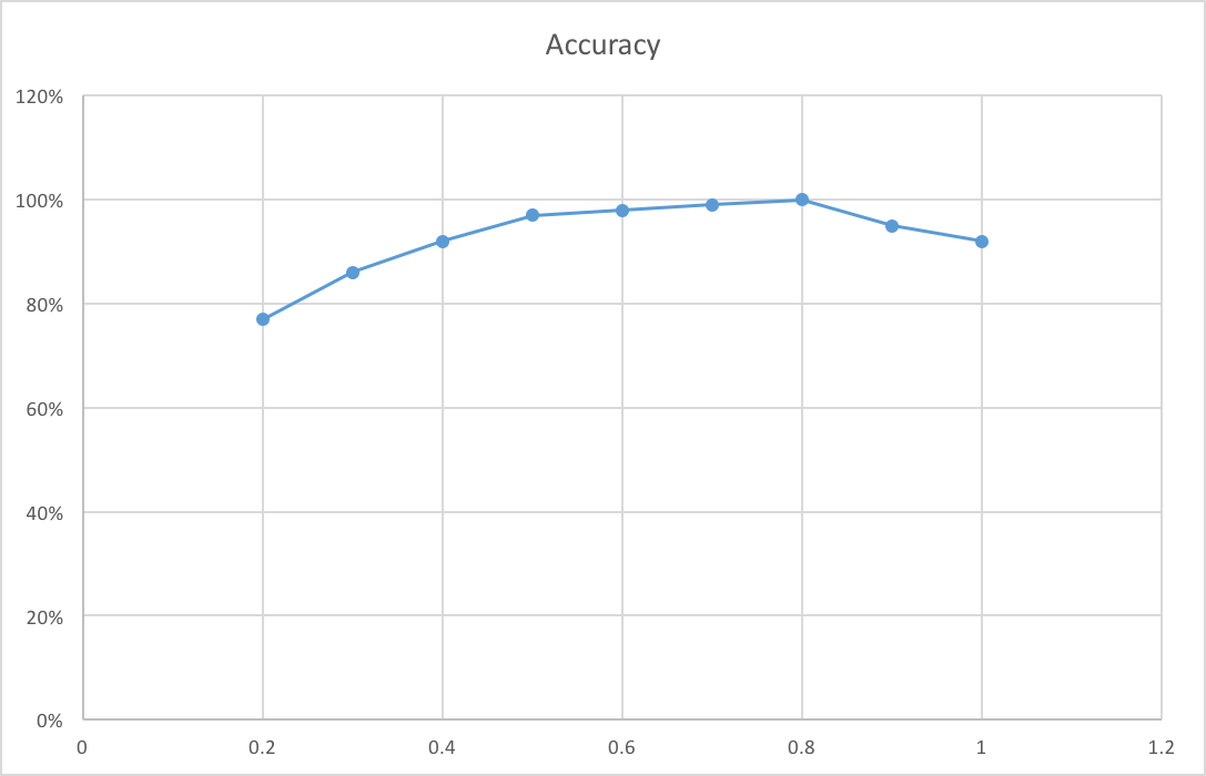
Fig 5. Relationship between accuracy and image scale.

Try the adaptive non-maximum suppression

It means that the interest points are not only the local maximal but also larger than their neighbors in a pretty large region. For the Notre Dame image pair, by implementing the ANMS, the number of interest point decrease to 1/3 and the accuracy of the top 100 increase from 90% to 97%.

Do experiment with differnt SIFT parameters

I try and figure out 128 will be the comparatively good feature size. If the feature become larger, it will contain more information and give better result. But it takes too long for the calulation. While small feature can not represent the point well.

Each histogram has 8 orientations and I add the magnitude to two nearest orientations instead of one.

For the feature normalization, I will first normalize it and the filter out those value which is larger than 0.2. At first, I didn't filter out value larger then 0.2 and get 91% accuracy for Notre Dame pair. But the filter boost the accuracy to 97% then. So the filter in the normalization is really important.


% Normalization
features(i,:)=features(i,:)/norm(features(i,:));
features(i,features(i,:)>0.2)=0.2;
features(i,:)=features(i,:)/norm(features(i,:));

Using kd-tree to accelerate matching

Taking the Notre Dame for example. There are 1678 interest points in image 1 and 1623 interest points in image 2. The feature matching time for the naive matching algorithm is 0.5154 second while the time for kd-tree structure is only 0.2828 second. It savee half of the time by using kd-tree


% naive implementation of algorithm
num=1;
distance=pdist2(features1,features2);
for i = 1:num_features
    if features1(i)~=zeros(1,128)
        [dists, index] = sort(distance(i,:),'ascend');
        confidence=dists(2)/dists(1);
        if (confidence>threshold)
            matches(num,:)=[i,index(1)];
            confidences(num,:)=confidence;
            num=num+1;
        end
    end
end
%% Elapsed time is 0.515488 seconds

%kd-tree implementation
kdtree=KDTreeSearcher(features2);
[index,dists] = knnsearch(kdtree,features1,'k',2);
num=1;
for i = 1:num_features
    if features1(i)~=zeros(1,128)
        confidence=dists(i,2)/dists(i,1);
        matches(num,:)=[i,index(i,1)];
        confidences(num,:)=confidence;
        num=num+1;
    end
end
%%Elapsed time is 0.282834 seconds

Result

Results for Notre Dame Image Pair

Fig 6. Ground truth evaluation result of Notre Dotre image pair. (Scale 0.5, feature_width:32, 97 total good matches, 3 total bad matches. 0.97% accuracy)

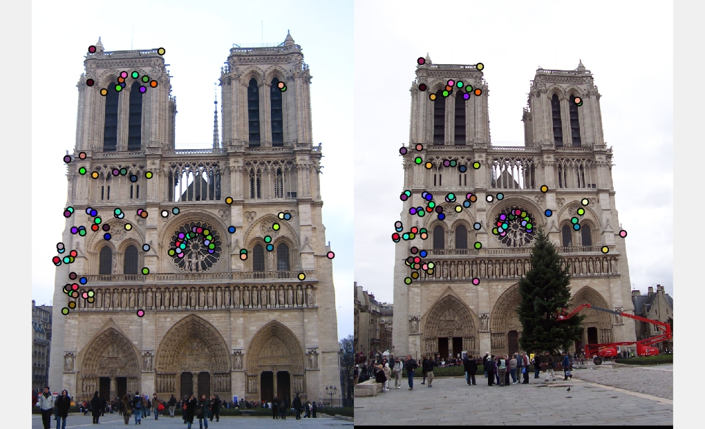
Fig 7. Interest Points Matching Results of Notre Dotre image pair. (Scale 0.5, feature_width:32, 97 total good matches, 3 total bad matches. 0.97% accuracy)

Results for Mount Rushmore Image Pair

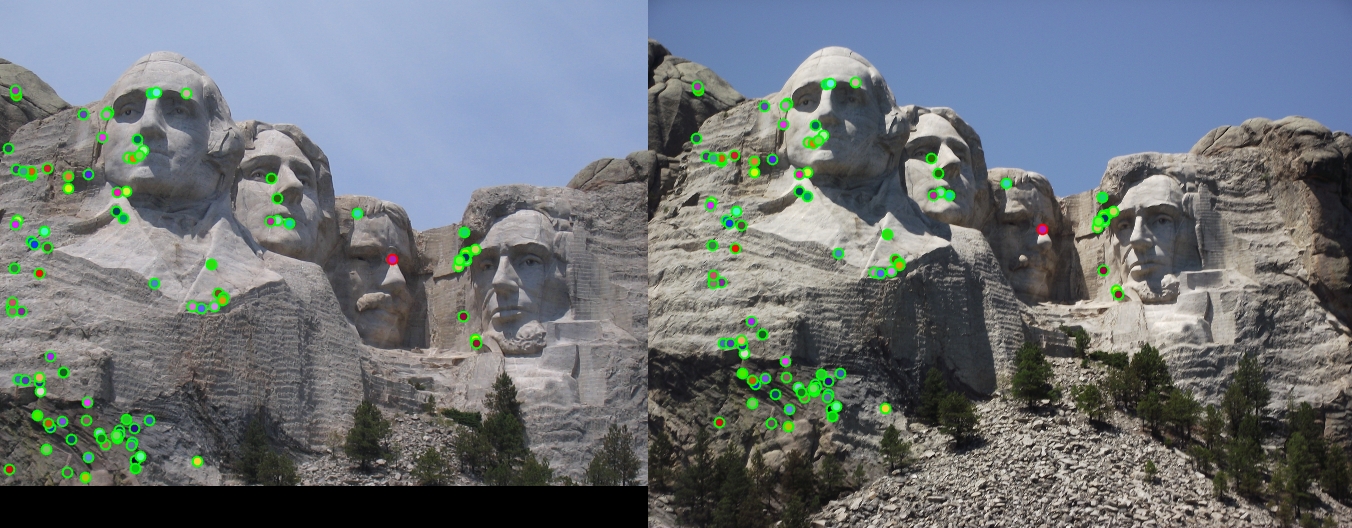
Fig 8. Ground truth evaluation result of Mount Rushmore image pair. (Scale 0.5, feature_width:32, 99 total good matches, 1 total bad matches. 0.99% accuracy)

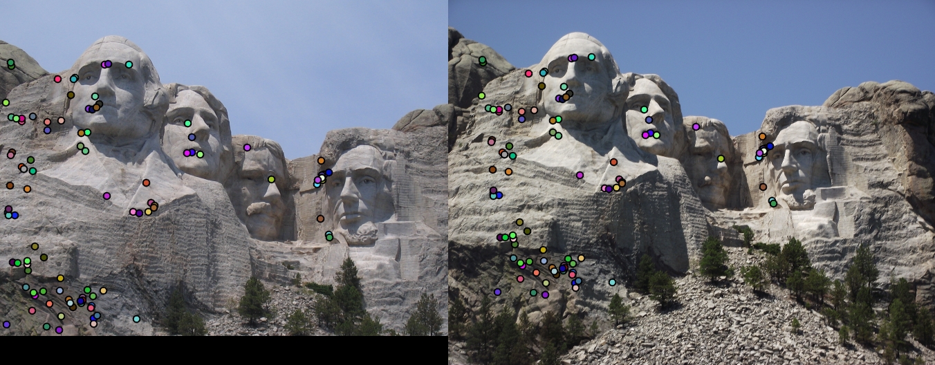
Fig 9. Interest Points Matching Results of Notre Dotre image pair. (Scale 0.5, feature_width:32, 99 total good matches, 1 total bad matches. 0.99% accuracy)

Results for Episcopal Gaudi Image Pair

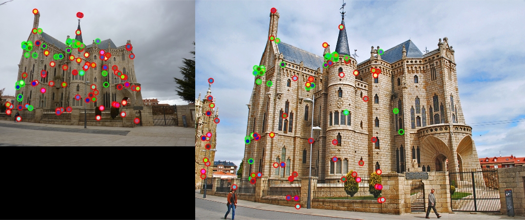
Fig 10. Ground truth evaluation result of Episcopal Gaudi image pair. (Scale 0.5, feature_width:64, 33 total good matches, 67 total bad matches. 0.33% accuracy)

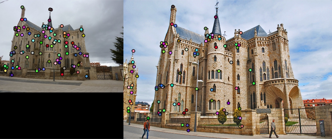
Fig 11. Interest Points Matching Results of Notre Dotre image pair. (Scale 0.5, feature_width:64, 33 total good matches, 67 total bad matches. 0.33% accuracy)

Results for Additional Image Pair

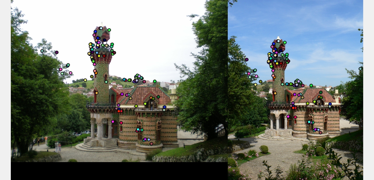
Fig 12. Ground truth evaluation result of Capricho Gaudi in Dot_color. (Scale 0.5, feature_width:32)

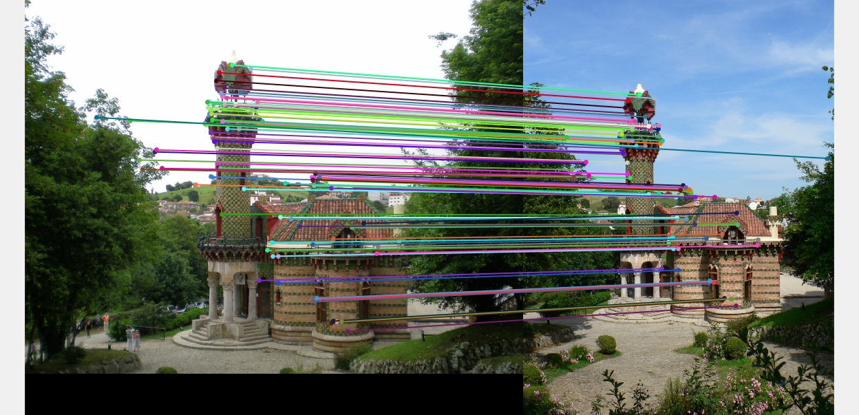
Fig 13. Ground truth evaluation result of Capricho Gaudi in arrow. (Scale 0.5, feature_width:32)

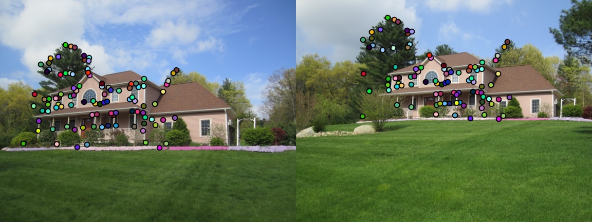
Fig 14. Ground truth evaluation result of House in Dot_color. (Scale 0.5, feature_width:32)

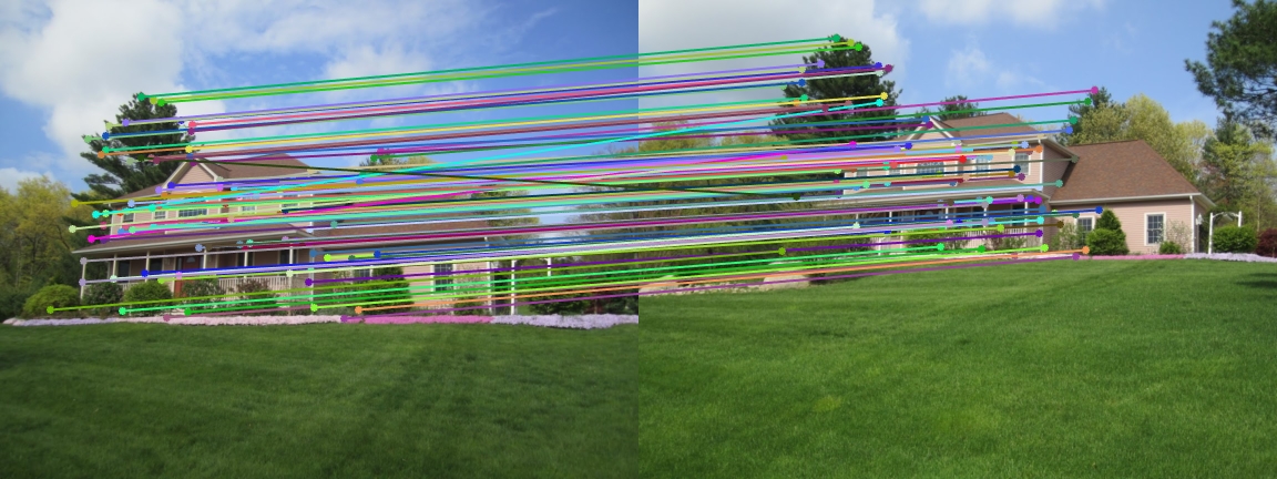
Fig 15. Ground truth evaluation result of House in arrow. (Scale 0.5, feature_width:32)

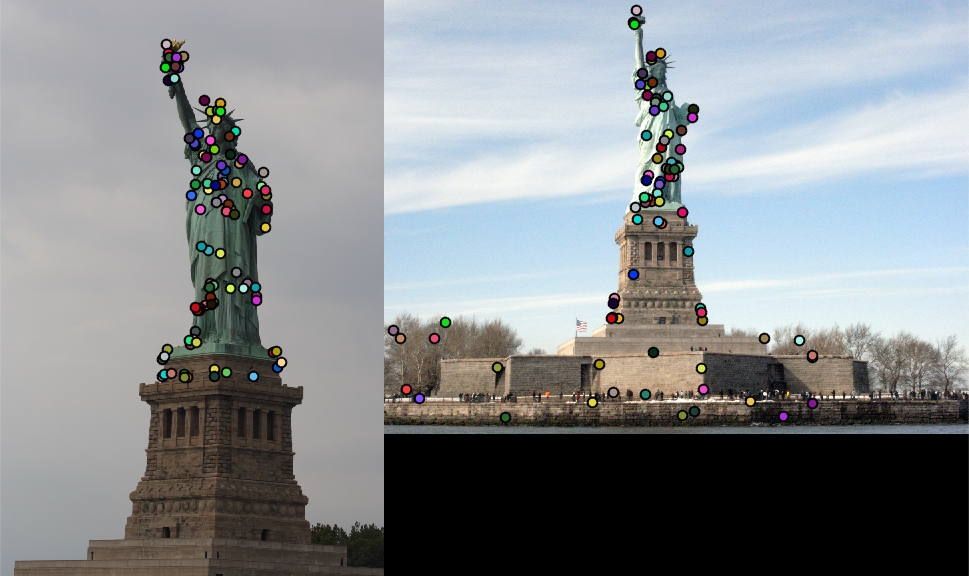
Fig 16. Ground truth evaluation result of Statue of Liberty image pair in Dot_color. (Scale 0.5, feature_width:32)

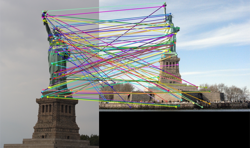
Fig 17. Ground truth evaluation result of Statue of Liberty image pair in arrow. (Scale 0.5, feature_width:32)

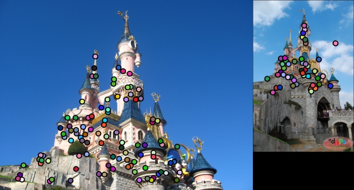
Fig 18. Ground truth evaluation result of Sleeping Beauty Castle Paris in Dot_color. (Scale 0.5, feature_width:32)

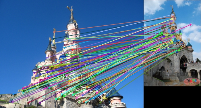
Fig 19. Ground truth evaluation result of Sleeping Beauty Castle Paris in arrow. (Scale 0.5, feature_width:32)

Jianling Wang 903143548

Project 2: Local Feature Matching