Name: Jia Wei GTID: 903149411

Example of a local feature matches.

Code and Algorithms

Interes Point Detection (get_interest_points.m)

The code shown below implements the Harris corner detector. The baseline Harris corner detector algorithm is:

1. Compute the horizontal and vertical derivatives of the image Ix and Iy by convolving the original image with derivatives of Gaussians
2. Compute the three images corresponding to the outer products of these gradients. (The matrix A is symmetric, so only three entries are needed.)
3. Convolve each of these images with a larger Gaussian
4. Compute a scalar interest
5. Find local maxima above a certain threshold and report them as detected feature point locations.

function [x, y, confidence, scale, orientation] = get_interest_points(image, feature_width)
    
[imagerow,imagecolumn]=size(image);

diff_Gaussian=fspecial('Gaussian',2)-fspecial('Gaussian',1);% Pre-defined Gaussian Matrix for differente dimensions
four_dim_Gaussian=fspecial('gaussian',4);

dx=[-1,0,1];
dy=[-1;0;1];

Fx=conv2(image,dx,'same');% Image derivatives: Calculate the derivatives fx
Fy=conv2(image,dy,'same');% Image derivatives:Calculate the derivatives fy

F_x=imfilter(Fx,diff_Gaussian);
F_y=imfilter(Fy,diff_Gaussian);

Fx_square=imfilter(F_x.^2,four_dim_Gaussian);%Smoothed squared image derivatives
Fy_square=imfilter(F_y.^2,four_dim_Gaussian);
Fxy=imfilter(F_x.*F_y,four_dim_Gaussian);

harris=Fx_square.*Fy_square-Fxy.^2-0.04*((Fx_square+Fy_square).^2);%Calculate the harris value

maxima=colfilt(harris,[3,3],'sliding',@max);% find local maxima

x=[];
y=[];
for a=1:imagerow
    for b=1:imagecolumn
        if (harris(a,b)==maxima(a,b)&& (harris(a,b)>0.001))% Free Parameter: interest response threshold
            x=vertcat(x,b);
            y=vertcat(y,a);
        end
    end
end
end

Local Feature Description (get_features.m)

In this part, a SIFT-like local feature is implemented. More specifically, it returns a set of feature descriptors for a set of interest points given by the previous sub-function. In this project, the parameter “feature width” is set to be a constant 16. The code below firstly calculates the gradient magnitude and direction of the given image. Then, the image is filtered by a Gaussian filter. A 16 by 16 window around the detected keypoint and a gradient orientation histogram are created by adding the weighted gradient value to eight orientation histogram bins. The resulting 128 feature vectors are normalized to unit length. At last, the feature vectors are once again normalized to unit length after doing the threshold calculation.

function [features] = get_features(image, x, y, feature_width)
[imagerow,imagecolumn]=size(image);

[Gmag,Gdir] = imgradient(imfilter(image,fspecial('gaussian')));%calculate Gradient magnitude and direction
Gmag=imfilter(Gmag,fspecial('gaussian'));
Gdir=imfilter(Gdir,fspecial('gaussian'));

features=[];

for n=1:size(x)%iterate every interest point
    histograms=zeros(4,4,8);% 4*4*8 histograms
    cell_first_row=y(n)-8;
    cell_last_row=y(n)+feature_width-1-8;
    cell_first_column=x(n)-8;
    cell_last_column=x(n)+feature_width-1-8;
    if ( cell_first_row>0 && cell_last_row<=imagerow && cell_first_column>0 && cell_last_column <=imagecolumn   )
        direction=mat2cell(Gdir(cell_first_row:cell_last_row,cell_first_column:cell_last_column),[4 4 4 4],[4 4 4 4]);
        magnitude=mat2cell(Gmag(cell_first_row:cell_last_row,cell_first_column:cell_last_column),[4 4 4 4],[4 4 4 4]);
        for a=1:4
            for b=1:4
                for new_row=1:4
                    for new_column=1:4
                        if( direction{a,b}(new_row,new_column)>=0&&direction{a,b}(new_row,new_column)<45   )
                            histograms(a,b,1)=histograms(a,b,1)+magnitude{a,b}(new_row,new_column);
                        end
                        if(direction{a,b}(new_row,new_column)>=45&&direction{a,b}(new_row,new_column)<90)
                            histograms(a,b,2)=histograms(a,b,2)+magnitude{a,b}(new_row,new_column);
                        end
                        if(direction{a,b}(new_row,new_column)>=90&&direction{a,b}(new_row,new_column)<135)
                            histograms(a,b,3)=histograms(a,b,3)+magnitude{a,b}(new_row,new_column);
                        end
                        if(direction{a,b}(new_row,new_column)>=135&&direction{a,b}(new_row,new_column)<180)
                            histograms(a,b,4)=histograms(a,b,4)+magnitude{a,b}(new_row,new_column);
                        end
                        if(direction{a,b}(new_row,new_column)>=-45&&direction{a,b}(new_row,new_column)<0)
                            histograms(a,b,5)=histograms(a,b,5)+magnitude{a,b}(new_row,new_column);
                        end
                        if(direction{a,b}(new_row,new_column)>=-90&&direction{a,b}(new_row,new_column)<-45)
                            histograms(a,b,6)=histograms(a,b,6)+magnitude{a,b}(new_row,new_column);
                        end
                        if(direction{a,b}(new_row,new_column)>=-135&&direction{a,b}(new_row,new_column)<-90)
                            histograms(a,b,7)=histograms(a,b,7)+magnitude{a,b}(new_row,new_column);
                        end
                        if(direction{a,b}(new_row,new_column)>=-180&&direction{a,b}(new_row,new_column)<-135)
                            histograms(a,b,8)=histograms(a,b,8)+magnitude{a,b}(new_row,new_column);
                        end
                    end
                end
            end
        end
    end
    
    fvector=reshape(histograms,[1,128])./norm(reshape(histograms,[1,128]));% build 128 D vectors and each feature should be normalized to unit length
    
    fvector(fvector>0.8)=0;%Free Parameters: feature vector threshold
    
    f_final=fvector./norm(fvector);% normalize again
    features=vertcat(features,f_final.^0.6);%raise each element of the final feature vector to some power that is less than one

end
end

Feature Matching (match_features.m)

In feature matching part, the nearest neighbor distance ratio test method of matching local features is implemented. To begin with, the Euclidean (vector magnitude) distances in feature space is directly used for ranking potential matches. Then NNDR is calculated to get the matches.

function [matches, confidences] = match_features(features1, features2)
features1_length=size(features1,1);
features2_length=size(features2,1);

matches=[];
confidences=[];

for a=1:features1_length
    for b=1:features2_length
        distance(a,b)=sqrt(sum((features1(a,:)-features2(b,:)).^2));%euclidean distance
    end
end

for a=1:features1_length
    sort_distance=sort(distance(a,:));
    NNDR=sort_distance(1)/sort_distance(2);%nearest and second nearest neighbor distances
    match_distance=find(distance(a,:)==sort_distance(1));
    if(NNDR<0.8) % Free parameter: nearest neighbor distance ratio
        matches=vertcat(matches,[a,match_distance(1)]);
        confidences=vertcat(confidences,1/NNDR);
    end
end

% Sort the matches so that the most confident onces are at the top of the
% list. You should probably not delete this, so that the evaluation
% functions can be run on the top matches easily.
[confidences, ind] = sort(confidences, 'descend');
matches = matches(ind,:);

Results and Discussion

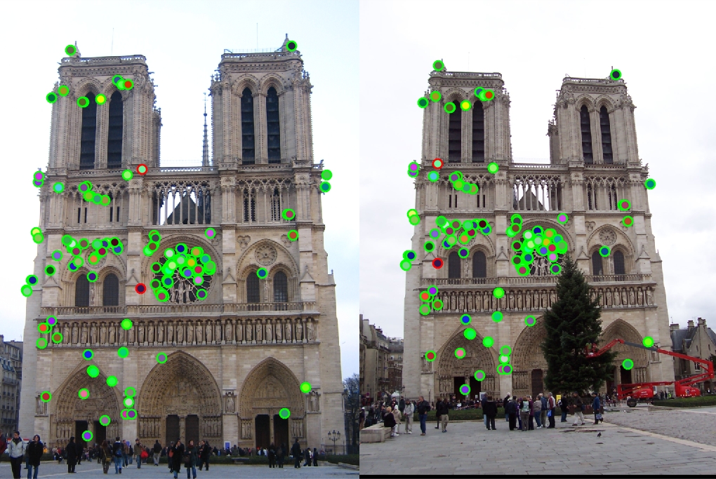
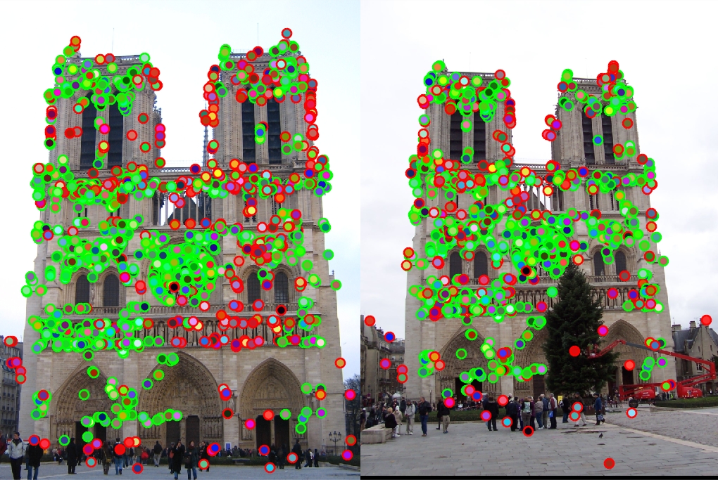
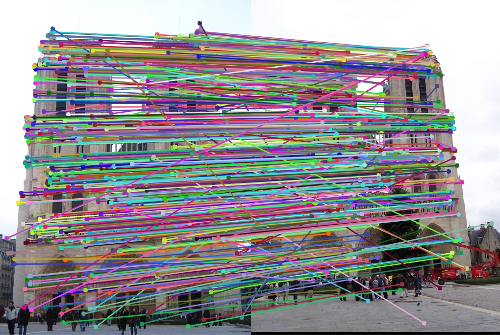
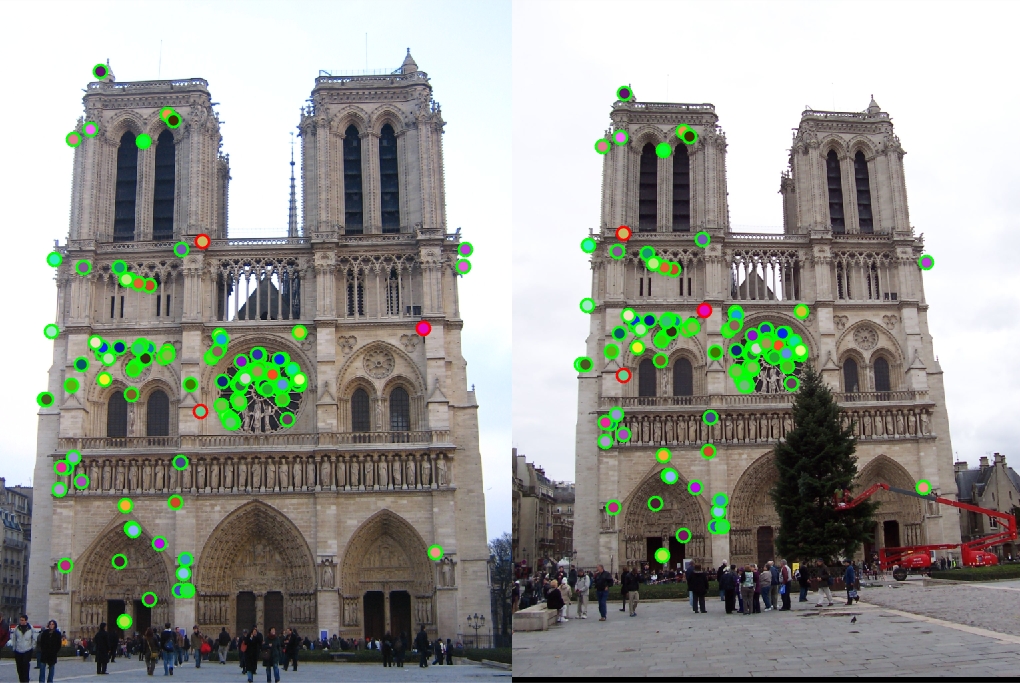
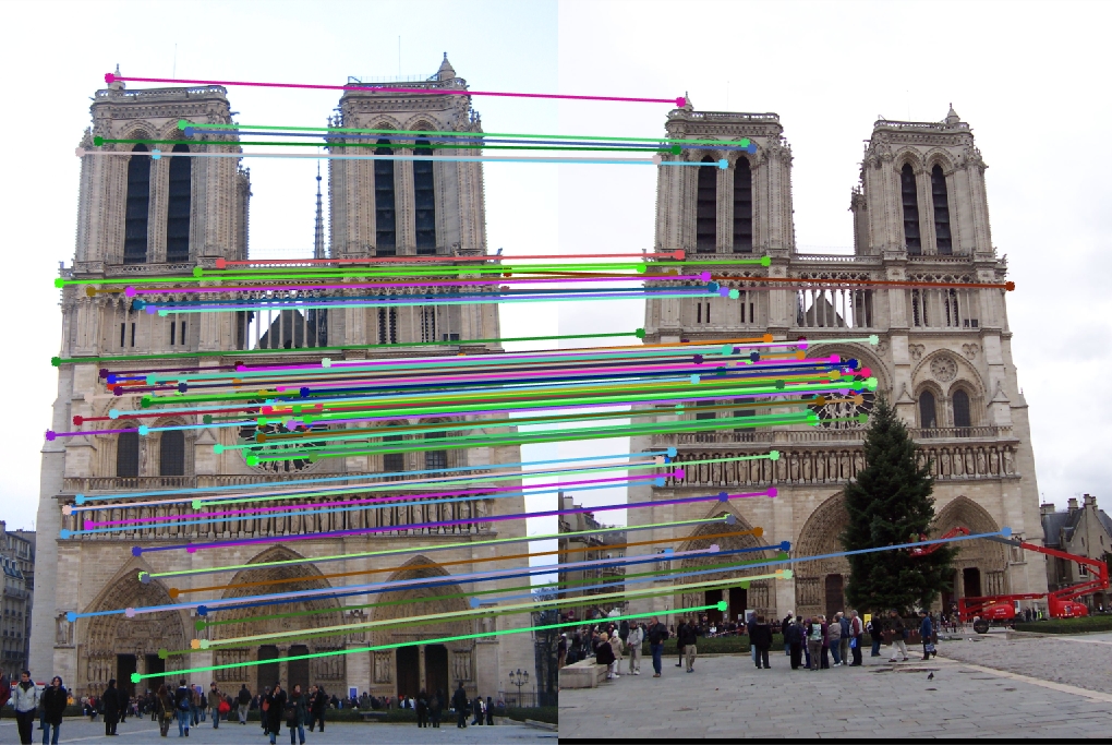
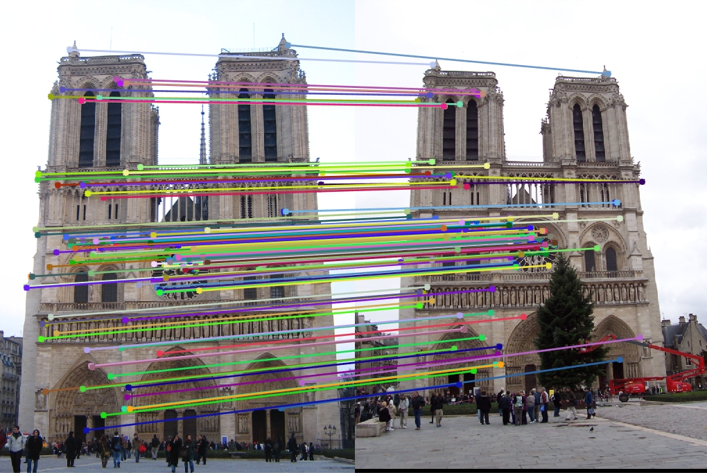
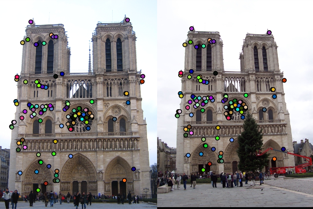
Notre Dame Results

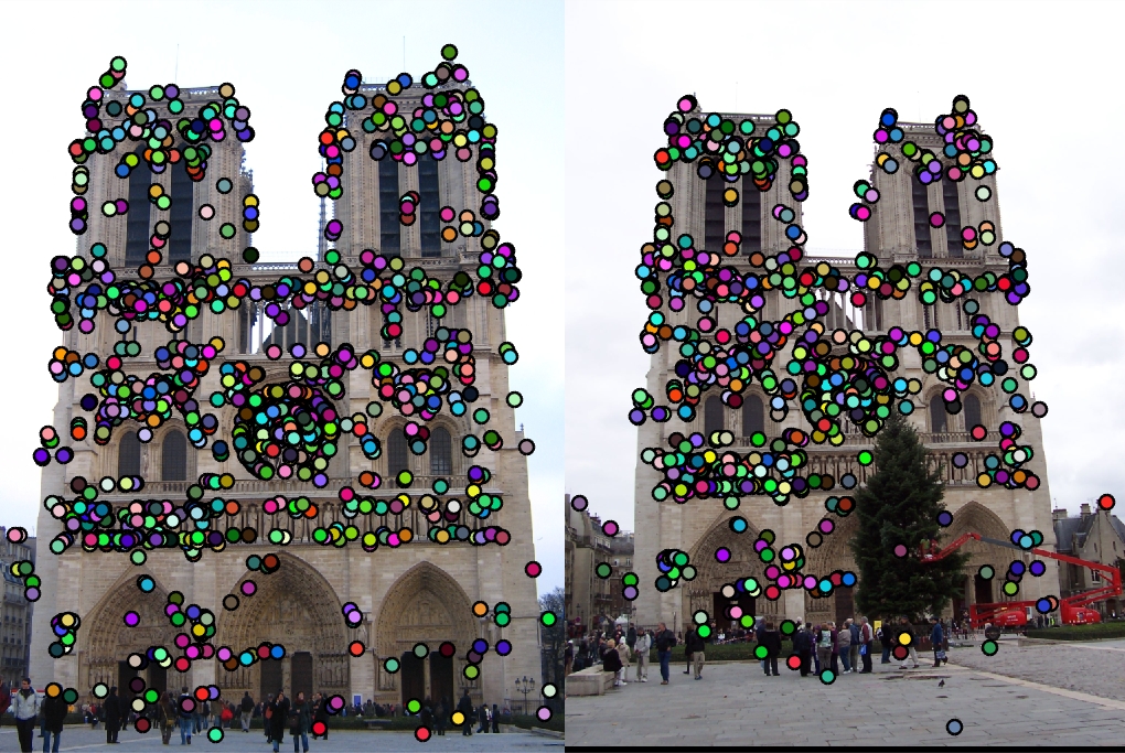Feature Vector Threshold = 0.5, NNDR = 0.9, 934 good matches, 323 bad matches, 74% accuracy

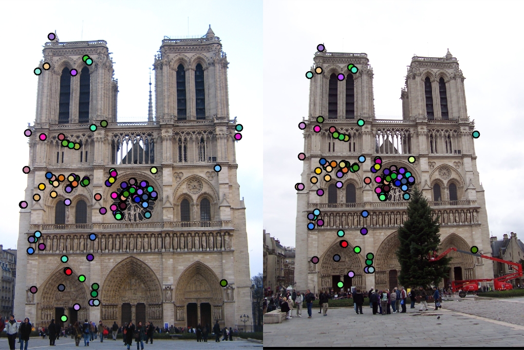Feature Vector Threshold = 0.5, NNDR = 0.7, 122 good matches, 3 bad matches, 98% accuracy

Feature Vector Threshold = 0.8, NNDR = 0.7, 137 good matches, 2 bad matches, 99% accuracy

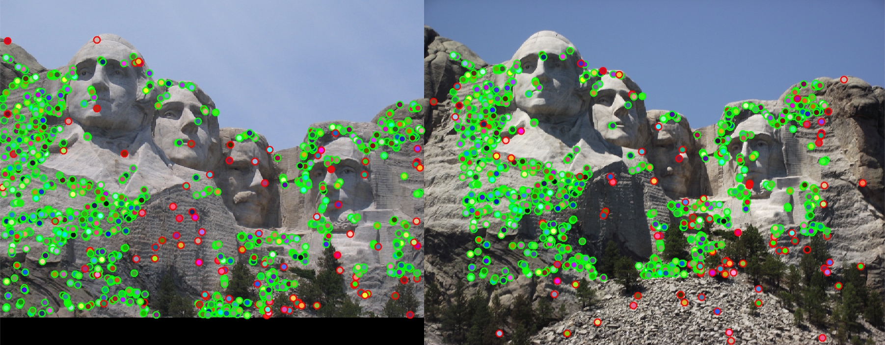
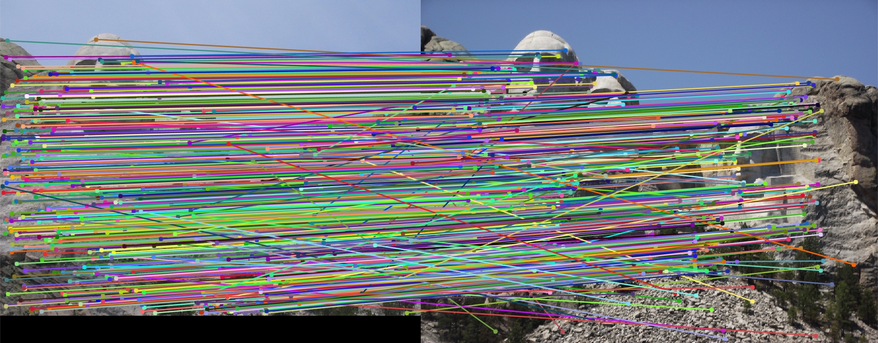
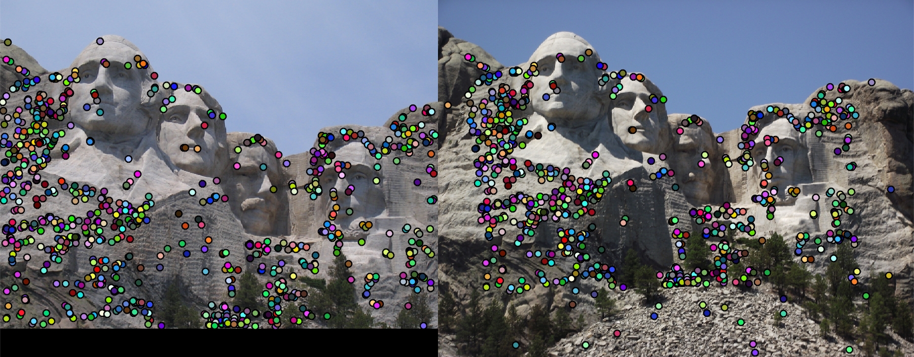
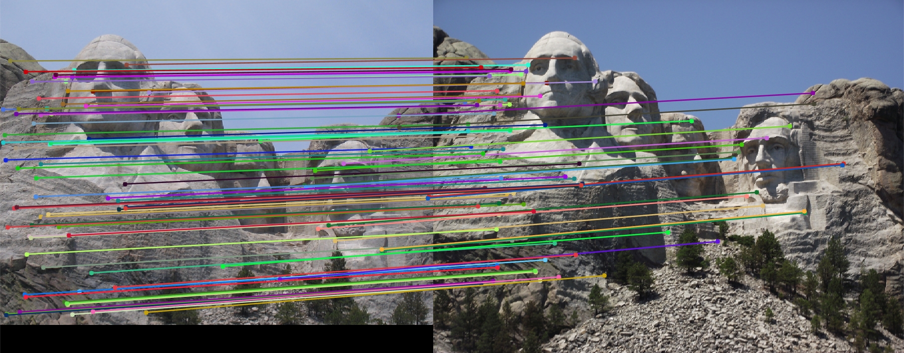
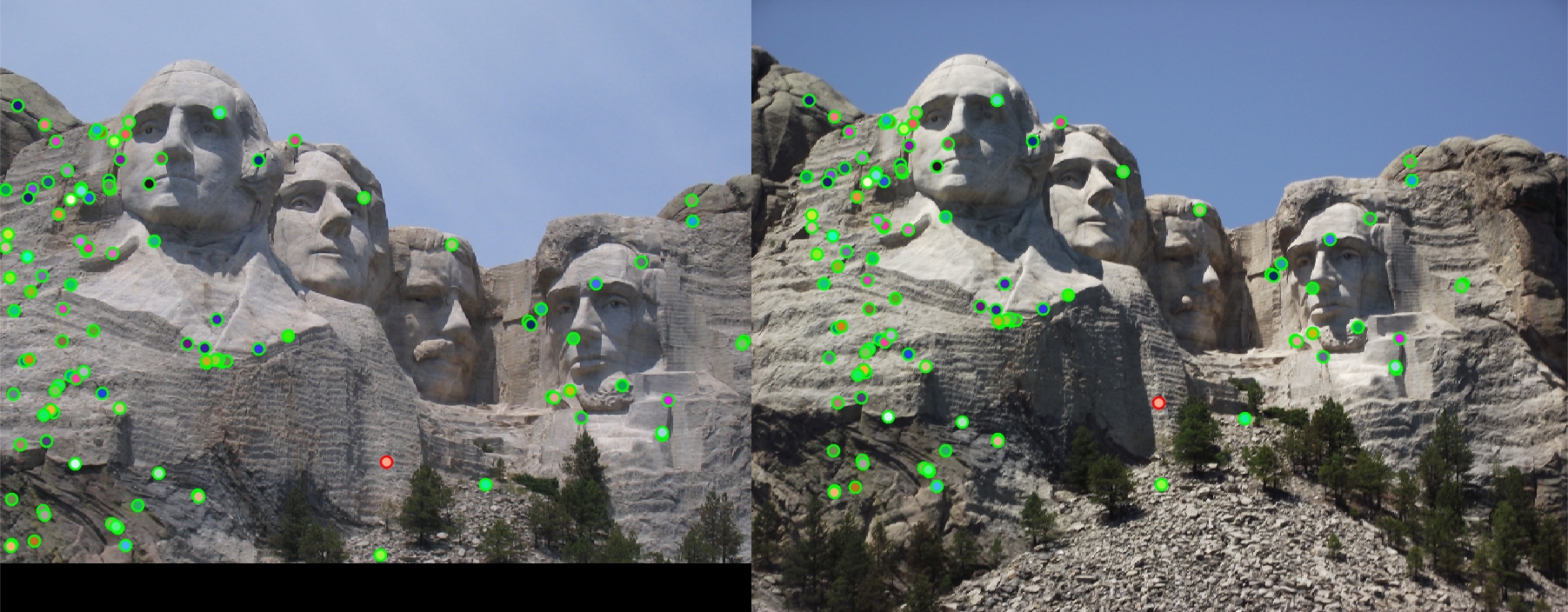
Mount Rushmore Results

Feature Vector Threshold = 0.5, NNDR = 0.9, 765 good matches, 97 bad matches, 89% accuracy

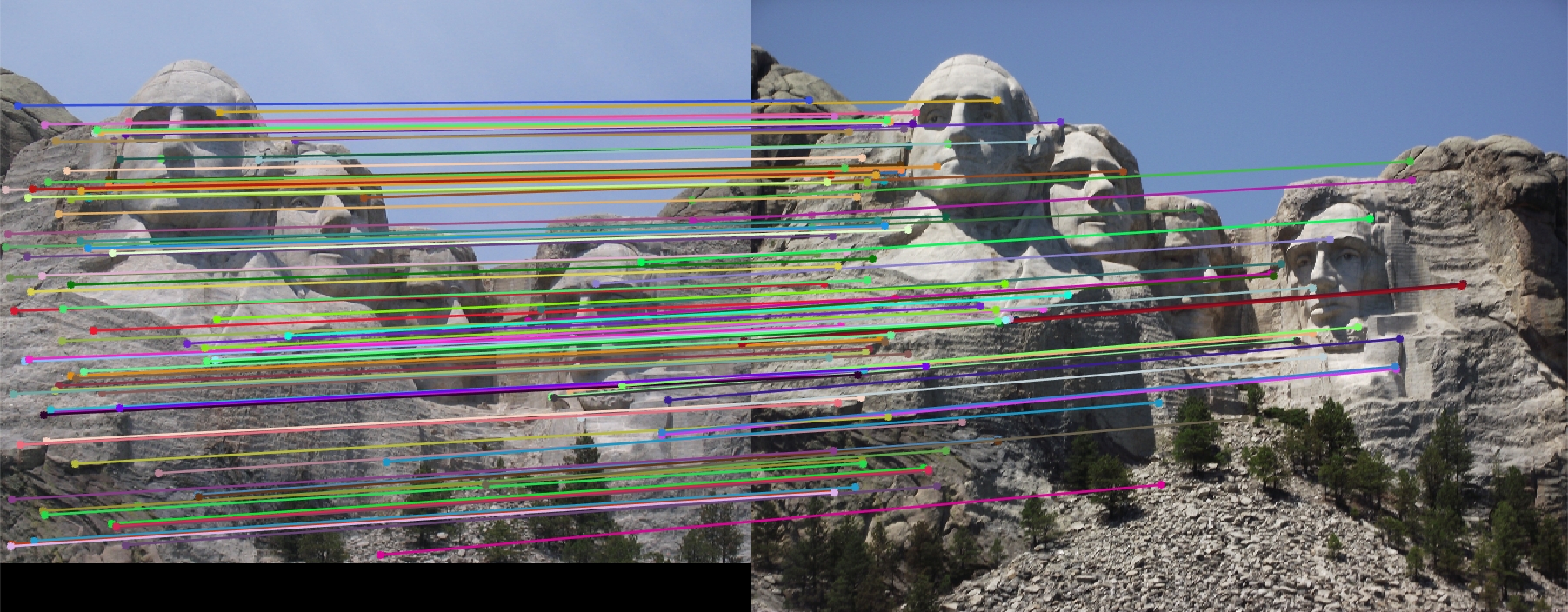
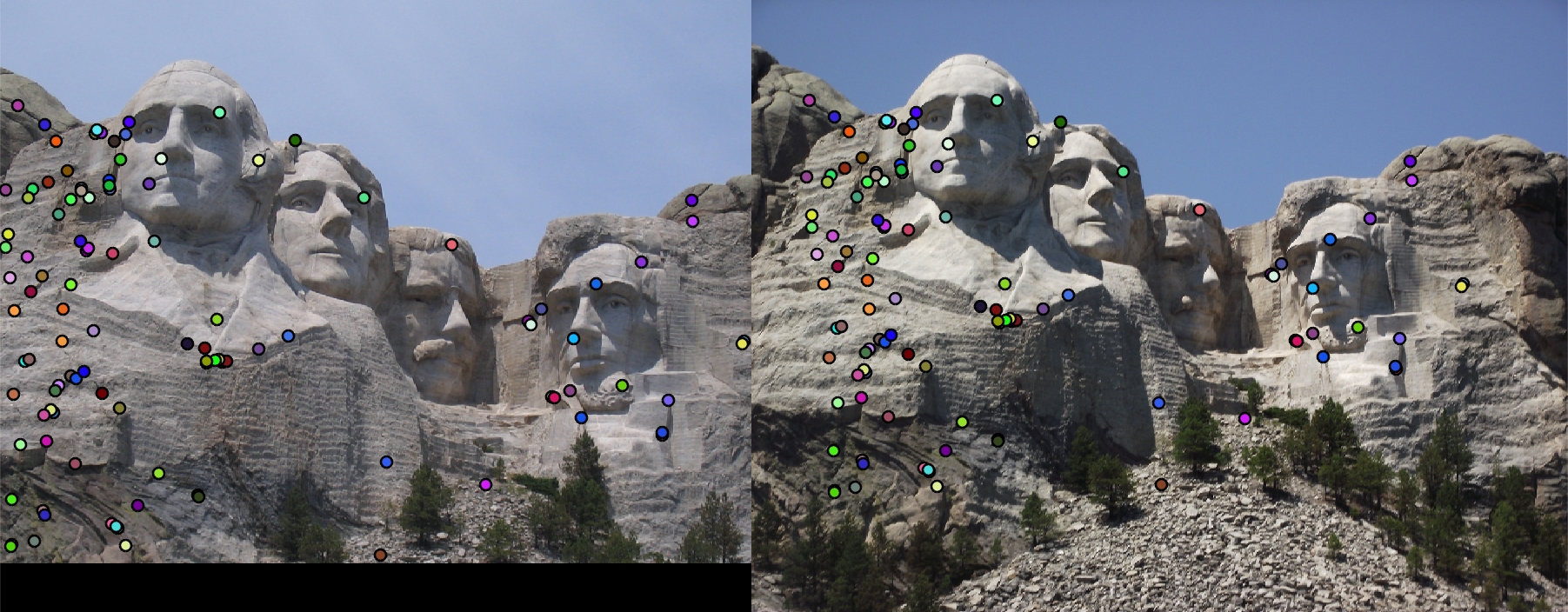
Feature Vector Threshold = 0.5, NNDR = 0.7, 85 good matches, 1 bad matches, 99% accuracy

Feature Vector Threshold = 0.8, NNDR = 0.7, 108 good matches, 1 bad matches, 99% accuracy

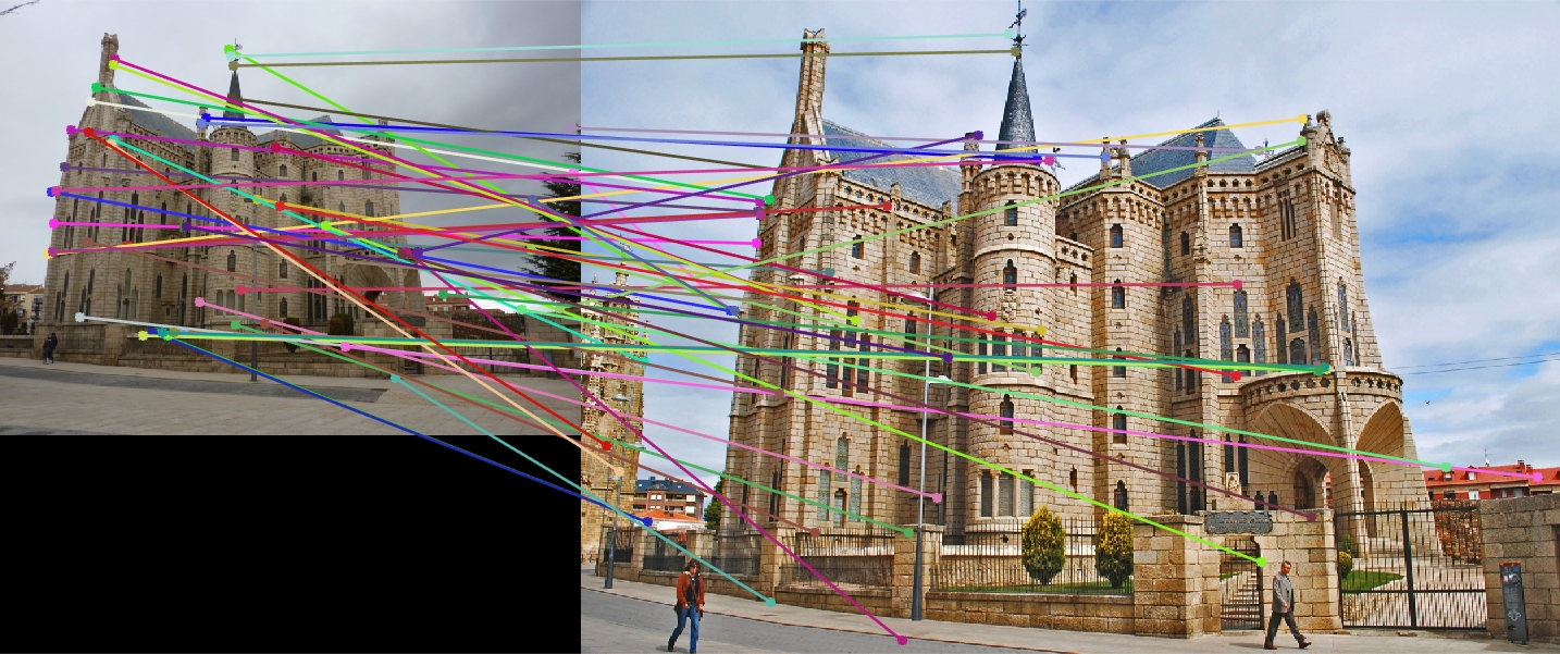
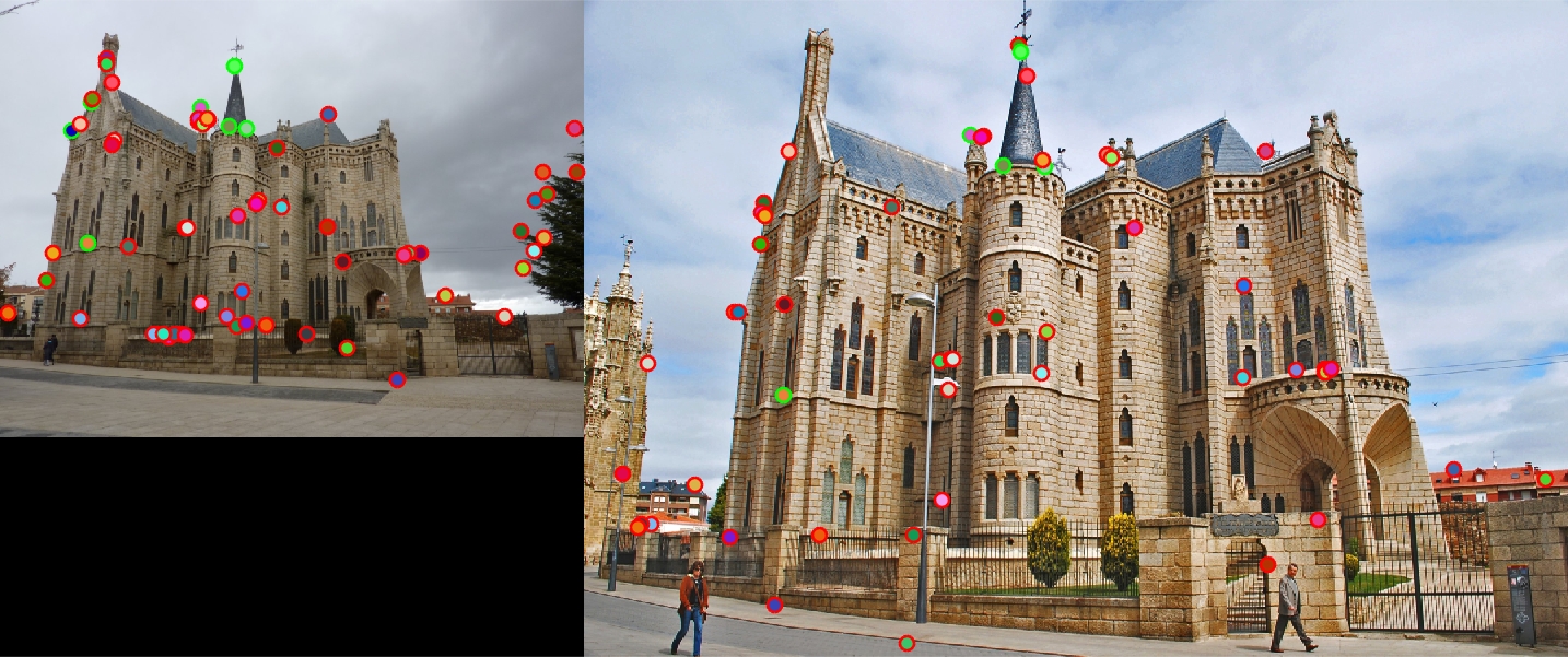
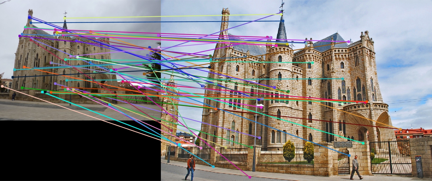
Episcopal Gaudi Results

Feature Vector Threshold = 0.5, NNDR = 0.9, 5 good matches, 50 bad matches, 9% accuracy

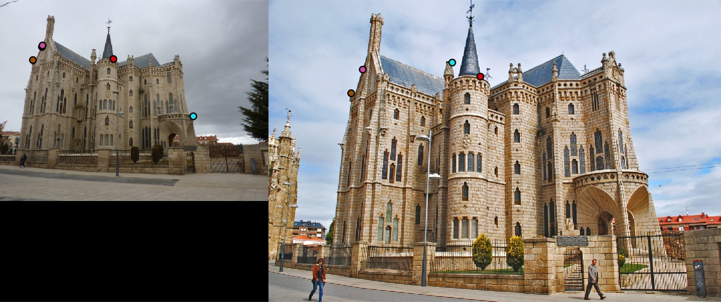Feature Vector Threshold = 0.8, NNDR = 0.8, 3 good matches, 2 bad matches, 60% accuracy

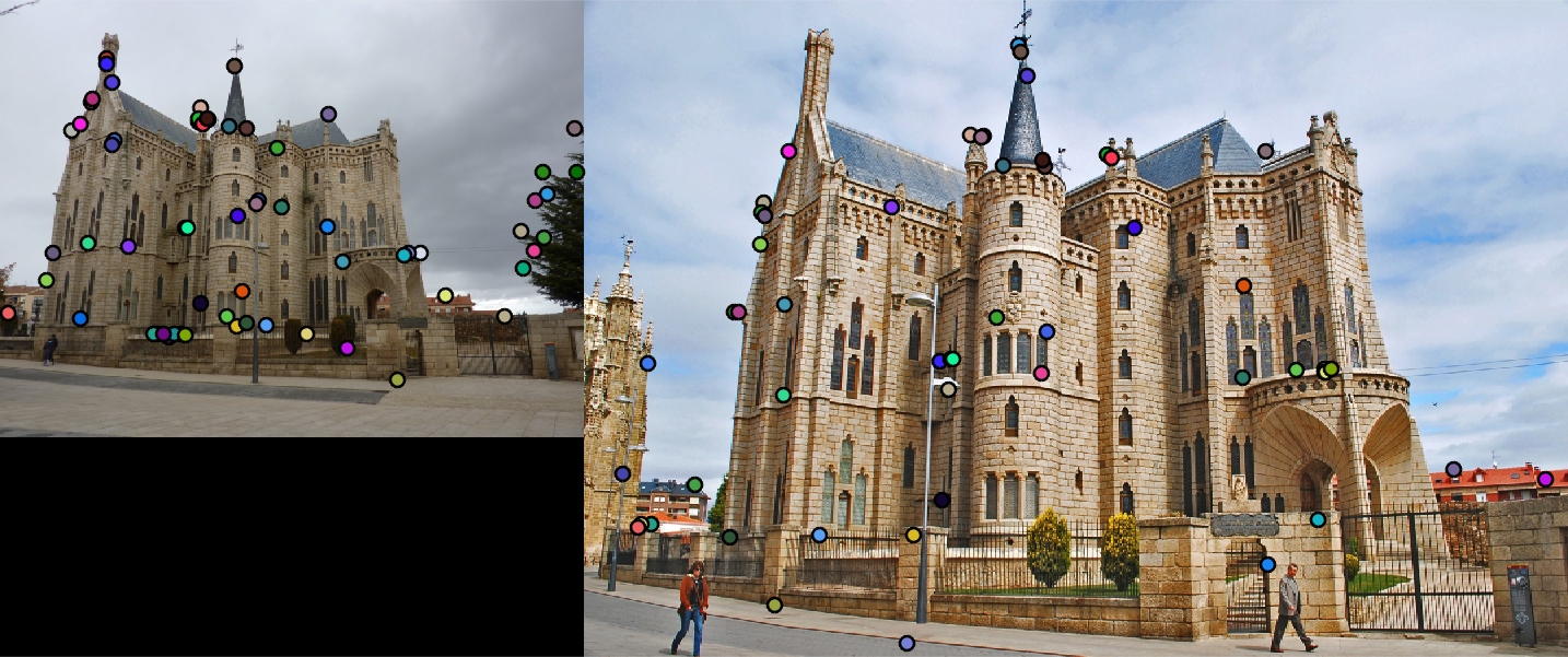Feature Vector Threshold = 0.8, NNDR = 0.9, 7 good matches, 57 bad matches, 11% accuracy

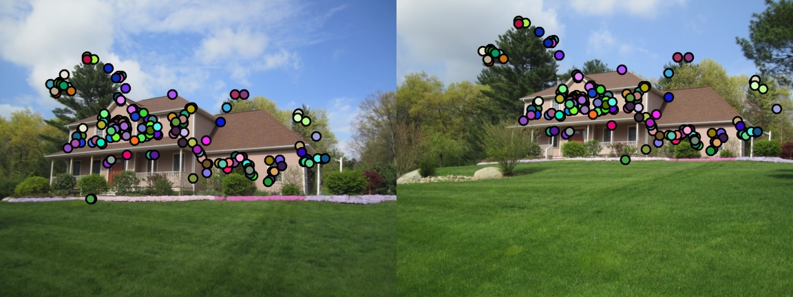
Some Extra Works

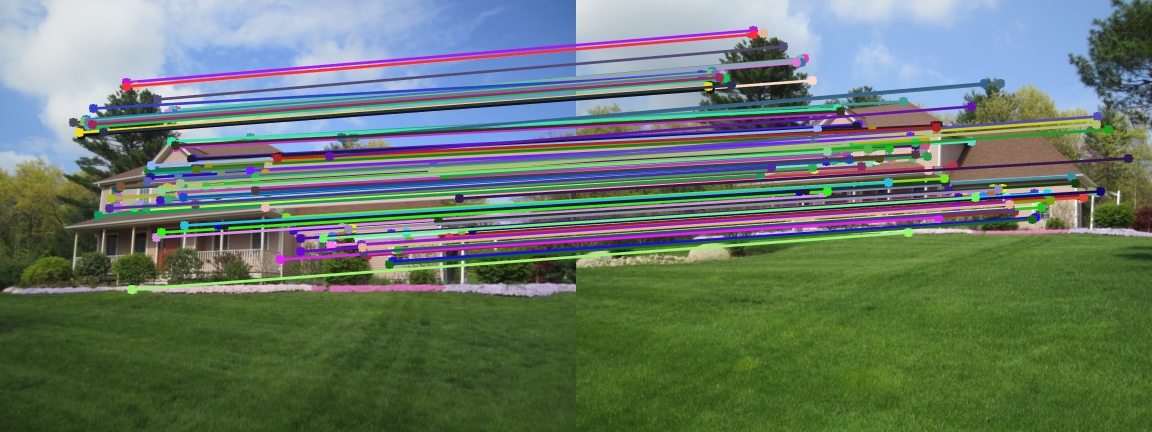GOOD: Image Pair: House. Feature Vector Threshold = 0.8, NNDR = 0.8

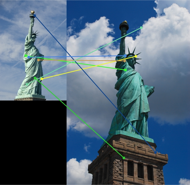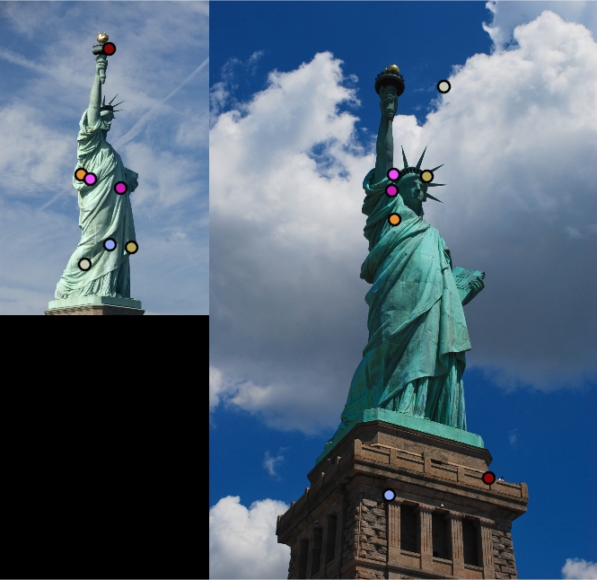
BAD: Image Pair: Statue of Liberty.Feature Vector Threshold = 0.8, NNDR = 0.8

In this part, several pairs of image in extradata file are used to test the above three functions. Although there are no eval (ground truth) file to illustrate the accuracy, it can be found that for House Image, the accuracy is quite high. The reason could be that the original image pair is very similar so it will not be hard to match certain interest points. However, for the below image pair Statue of Liberty, the accuracy, by observing, is relatively low. The reason can be the threshold value for finding interest points and the threshold value for matching features (NNDR) are too high for this image pair.

Discussion

In this project, for the Notre Dame image pair, first of all, the accuracy is relatively low. Then, according to the instruction in get_features.m, each element of the final feature vector is raised to the power of 0.6. Then, the feature vector threshold is set to be 0.5 and NNDR is set to be 0.9. The result, as shown above, generates a large amount of interest points and the accuracy is still not satisfactory. Next, the NNDR is decreased to 0.7 to reduce the number of interest point pairs. For this time, the result gets 122 good matches and 3 bad matches, and the accuracy increases to 98%. For the third time, the NNDR remains 0.7 but the feature vector threshold is increased to 0.8 in order to increase the amount of interest points. The accuracy gets higher to 99%. For the image pair of Mount Rushmore, the similar results can be achieved. For Episcopal Gaudi, when the Feature Vector Threshold is set to be 0.8 and NNDR is set to be 0.8, the result gets 3 good matches and 2 bad matches. The result is not applicable since there is not enough interest points. When the feature vector threshold is set to be 0.8 and NNDR is set to be 0.9, the accuracy increases to 11%, with 7 good matches and 57 bad matches.