Project 2: Local Feature Matching
Example of a right floating element.
Feature detection and matching are are used by many computer vision applications. It can be used for checking the in between view for constructing the three dimentional image. The two matching images can be attached to form a mosaic.
There are following phases in the whole pipeline.
- Get interest points
- Extract features from the obtained interest points
- Match the features
- Obtain the complete mapping of the interest points
- Get interest points
- Create a window in the image matrixs
- In the above step, take care of the boundry interest points by skipping the edges
- find the points surrounding the window with the values more than the threshold.
- Non maximum supression. Here find the lcoal maximas.
- Store the interest points above the threshold into a vector
- Extract features from the obtained interest points
- Consider each interest point and take 16*16 patch surrounding it.
- Calculate gradients for each pixel by using imgradient
- Divide the patch into 4*4 cells
- Form Histogram by creating 8 bins. Classify each pixel gradient in the bin
- Store the histogram in the feature vector
- Normalise the histogram.
- Match the features
-
KD tree implementation
As extra credit assignment KD tree is implemented with KNN search. It generate KD trees for finding the nearest neighbour and stored into and array.
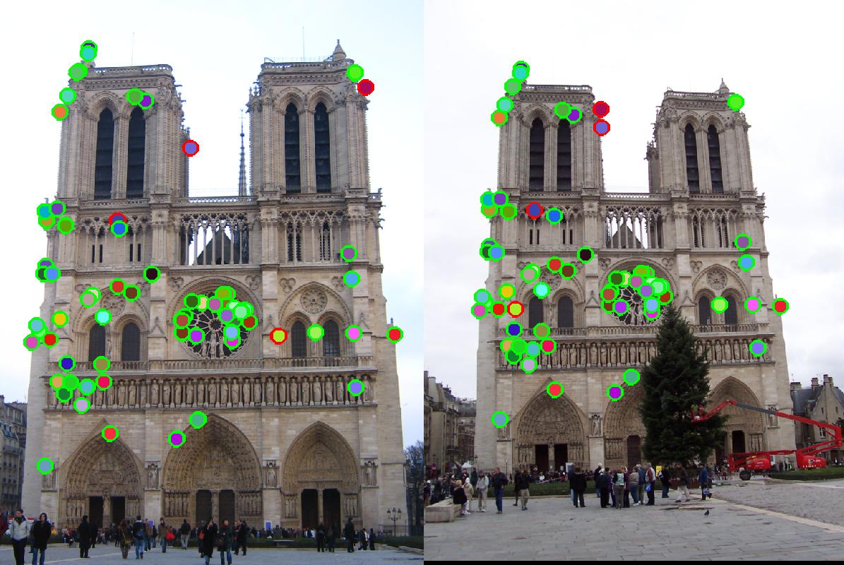
For the first point mentioned above, we need to find the points on the image that are distinct and can be used to find individual element which can be used to indentify the image. Thus when we look at the images, the parts which are plain are not useful. We need to look at the intersections or edges. Here comes the concept of edge detection and founding the boundries. Various algorithms can be used for this purpose. In the implementation, Harris corner detection is implemented. Harris corner detection involves finding the horizontal and vertical gradient. Following are the steps involved in Harris corner detection:
%Harris corner detection
filter1 = fspecial('gaussian', [3 3], 0.5);
image = imfilter(image,filter1);

[Ix, Iy] = imgradientxy(image);
%imgradientxy create gradients in horizontal and vertical direction

Ixx = Ix.*Ix;
Iyy = Iy.*Iy;
Ixy = Ixx.*Iyy;
new_image = Ixx.*Iyy - Ixy.*Ixy - sigma*(Ixx + Iyy).*(Ixx + Iyy);
%Point 4 in the slide:  Cornerness function. Second equation


filter2 = fspecial('gaussian',[7 7], 0.5);
new_image = imfilter(new_image,filter2);
%filter again
The second part involves extracting the features from the interest points. This is done in get_interest points function. Here the interest points are processed to get the unique features in them. In the first part of the assignment, patches surrounding the interest points were collected and normalised to get the feature for that interest point.
In the second part, Scale Invarient Feature Transform is implemented. Here the patches surrounding the interest points are processed further. 16*16 matrix is taken as one path. It is further divided into 4*4 cell. The gradient and magnitude is calculated at each pixel in the 4*4 cell. The gradient is then classified into 8 orientation. The resulting into 4*4*8 feature points for each interest point.
%example code
    count=1;
    [row_x,row_y]=size(x);
    [row,column]=size(image );
    for x1= 1:1:row_x
        x_coor = x(x1);
        y_coor = y(x1);

        subset_image=image(y_coor-(feature_width/2):y_coor+((feature_width/2)-1)
			,x_coor-(feature_width/2):x_coor+((feature_width/2)-1));
			%create image patch as subset of the image.

        [imag,igrad]=imgradient(subset_image);
			%find the image gradient


        for i=0:feature_width/4:feature_width-(feature_width/4)
            for j=0:feature_width/4:feature_width-(feature_width/4)


                for m=1:1:feature_width/4
                    for n=1:1:feature_width/4

                        magnitude= imag(j+n,i+m); %magnitude at the pixel
                        angle= igrad(j+n,i+m);    %gradient at the pixel

                        if angle <45 && angle>=0
                            bin(1)=bin(1)+magnitude;
					%add magnitude to the bin if feature gradient falls in the bin
                        elseif angle <90 && angle>=45
                            bin(2)=bin(2)+magnitude;
                       ...
		       ...		%Same for 8 bins


                        end
                    end
                end

                appending_array=[appending_array bin(1) bin(2) .. bin(8)];
		%append the bins to feature
            end
        end


        features(count,:)=appending_array/sum(appending_array);
	%normalise
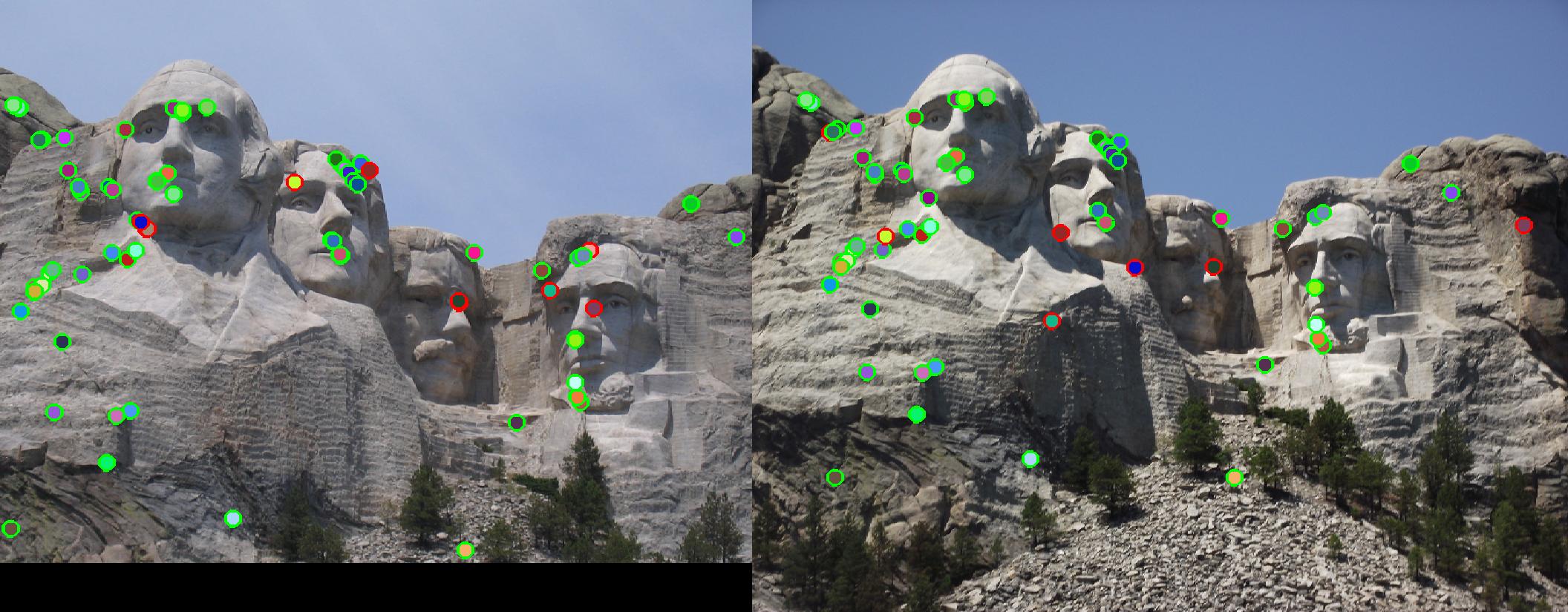
In the third part, the features between the two images are matched. Euclidian distace is taken between the feature points. Nearest neighbor ratio is calculated by considering the minimum and the second minimum of the features. The value is stored in the confidence vector and the matched feature points are stored in the matches matrix.
Results in a table
|
|
Results
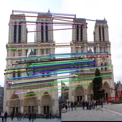
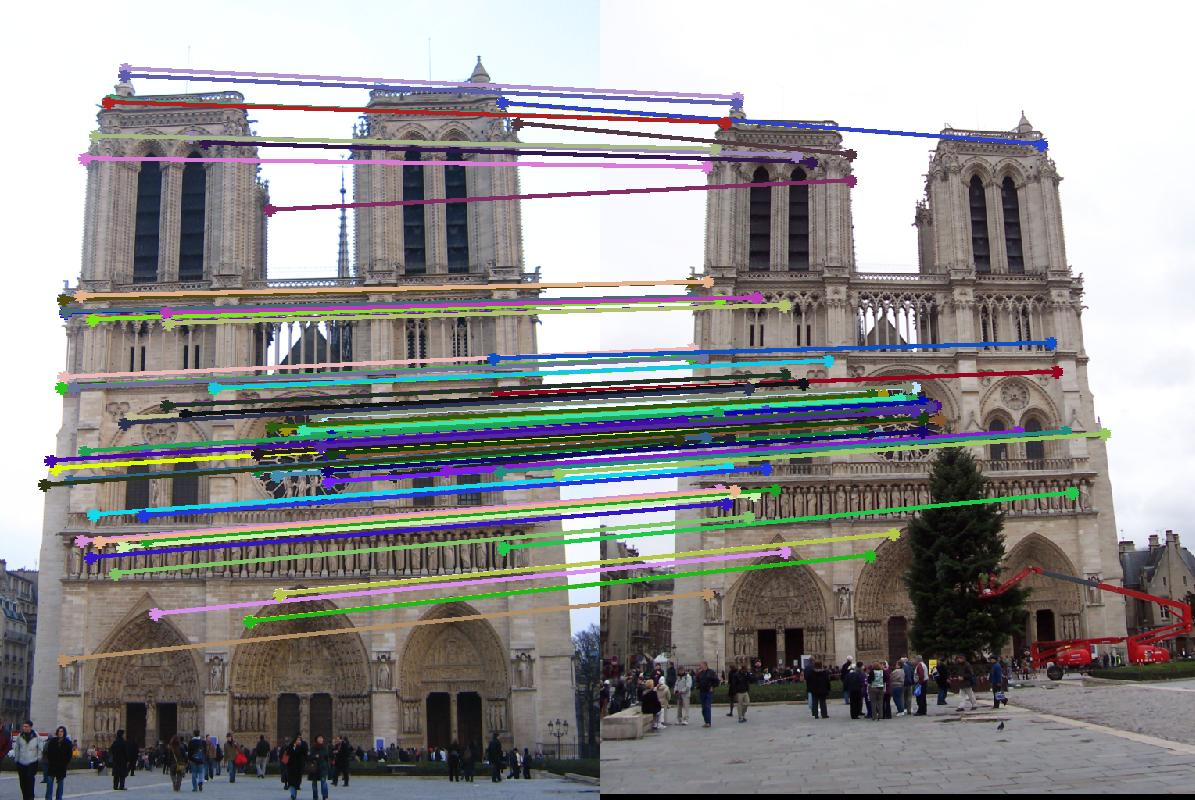
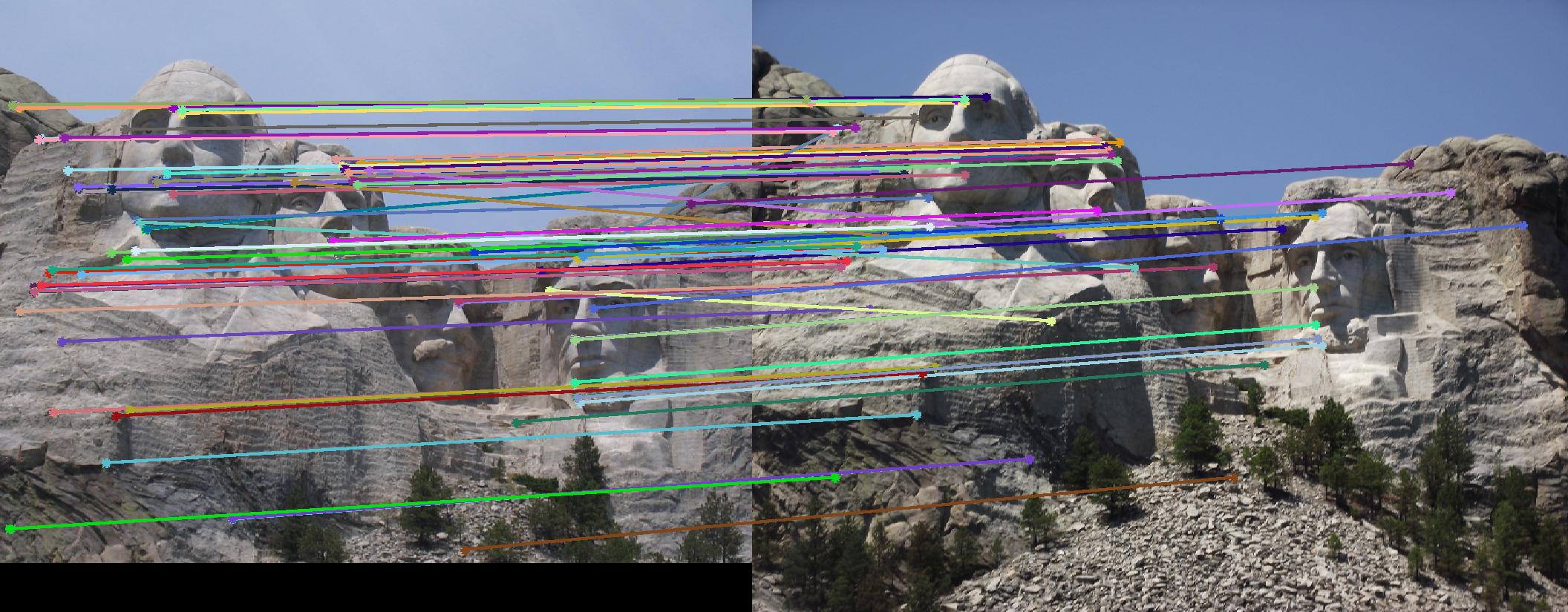
For Notre Dame,with the normalizes patch implementation, the accuracy was 56 % . With the SIFT features it went till 93%. And for Mount Rushmore it went to 83%.