Project 2: Local Feature Matching
This goal of this project was to create a local feature matching pipeline as follows:
- Find interest points using Harris corner detection
- Create local feature descriptors using SIFT feature descriptors
- Match features using the Nearest Neighbor Distance Ratio (NNDR)
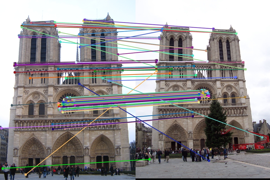
Feature matches between two images of the Notre Dame.
Harris Corner Detector
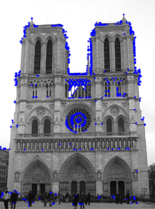
Interest points on the Notre Dame.
A Harris corner detector was implemented to find points of interest in the images. Interest points have a "cornerness" score above a threshold according to the Harris algorithm. In the textbook this value is 10000, but I modified my algorithm to choose points above 1 standard deviation of the mean value. This proved to be more effective than tuning a hard threshold because images differ in intensities, matrix data types, and number of corners
After thresholding the image, local maximum values were found within connected regions using the imregionalmax function. The x and y values of the maxima are then returned as interest points. This function proved to be more effective (10-15% higher) than using bwconncomp or bwlabel.
% Create Harris matrix
har = (gIx2 .* gIy2) - (gIxy .^ 2) - alpha * ((gIx2 + gIy2) .^ 2);

% Flatten matrix to find mean and sigma
flat = reshape(har, [], 1);
m = mean(flat);
sigma = std(flat);
% Remove values below first standard deviation
har(har<(m+sigma)) = 0;
...

% Get regional maximum points
regmax = imregionalmax(har);
[y, x] = find(regmax);
SIFT Feature Descriptors
A simple SIFT feature descriptor was created for each interest point. Initially I used a normalized patch as a feature descriptor, which resulted in 67% accurate matches when returning the 100 most confident matches. After implementing the SIFT feature descriptor the accuracy went up to 81%.
The SIFT feature descriptor was created by extracting a patch from the image, and applying a guassian filter to smooth the it. The gradient was then taken, and the magnitudes were weighted with gaussian weight to discount exterior pixels. The patch was divided into a 4x4 grid, and each gradient weight was binned into an a single orientation in a single quadrant. The end result was normalized and added to a list of features.
% Extract 16x16 window from image
window = image(y(i)-half_width:y(i)+half_width-1, x(i)-half_width:x(i)+half_width-1);
...
% After padding, smoothing, and cropping the window
[Gmag, Gdir] = imgradient(cropped);
...
% Downweight exterior gradient magnitudes with a gaussian weight
downweightGaussian = fspecial('gaussian', feature_width, half_width);
Gmag = Gmag .* downweightGaussian;
Nearest-Neighbor Feature Matching
To match features between images, the Nearest Neightbor Distance Ratio was computed for each feature. The Euclidean distance was found between each feature in image 1 with each feature in image 2, and the confidence was the ratio of the distance from the closest to second-closest neighbor. Confidence increases as the ratio approaches 0.
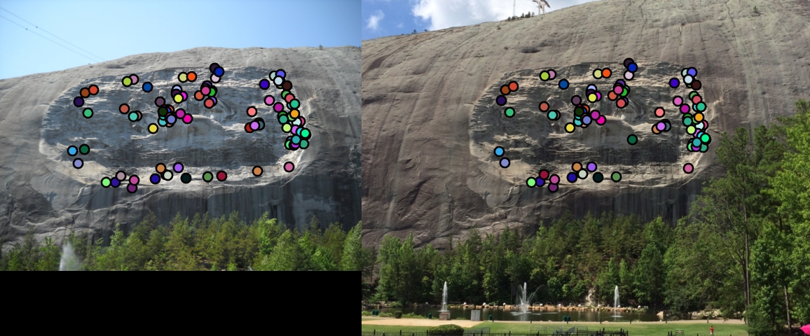
Feature matches on Stone Mountain.
The confidence-match tuples were sorted and only the 100 most confident were returned, producing 81% accuracy on the Notre Dame image. If only those with confidence less than 0.6 were returned instead, the accuracy of matches would increase to 94%, but with only 36 matches. This threshold of 0.6 was chosen from the following slide, which shows that the number of true positives decreases rapidly past that point. Thresholding in this way increases accuracy more predictably, but with fewer returned matches. For example, it returns 0 matches on the Episcopal Gaudi image.
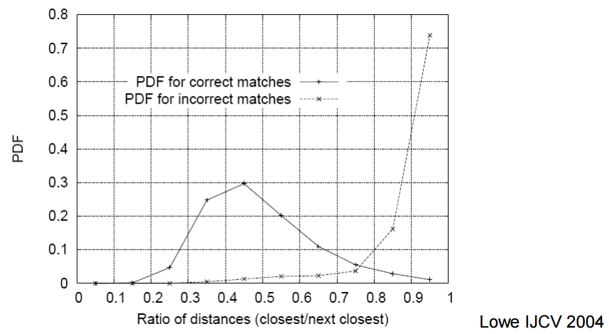
Probability density function of NNDR.
Results
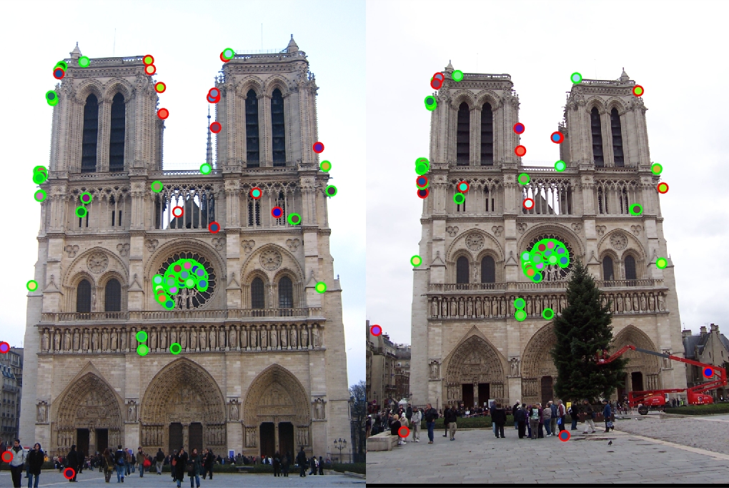
Notre Dame evaluation (81%).
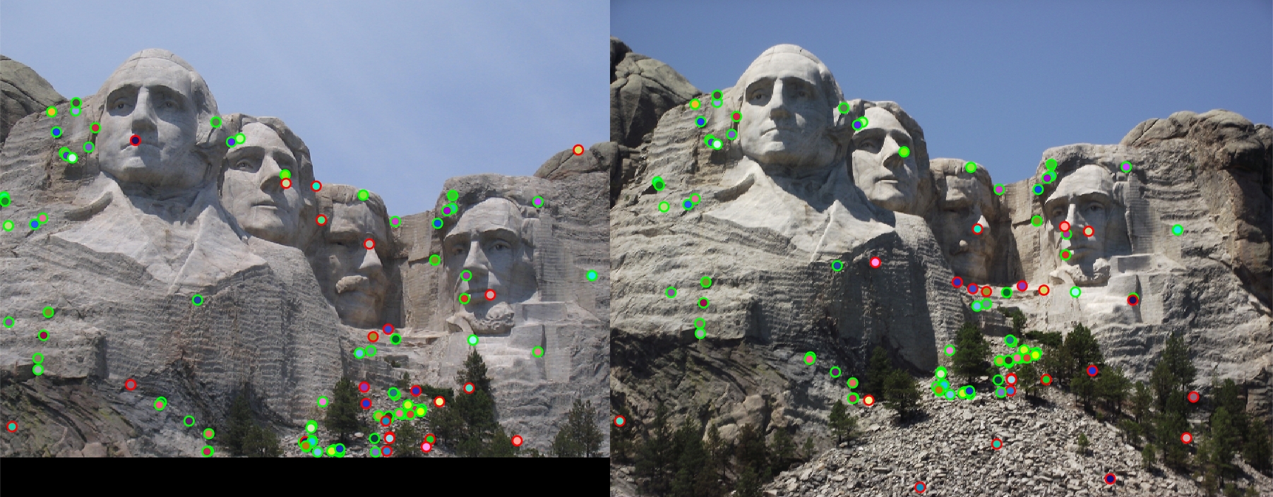
Mount Rushmore evaluation o (76%).
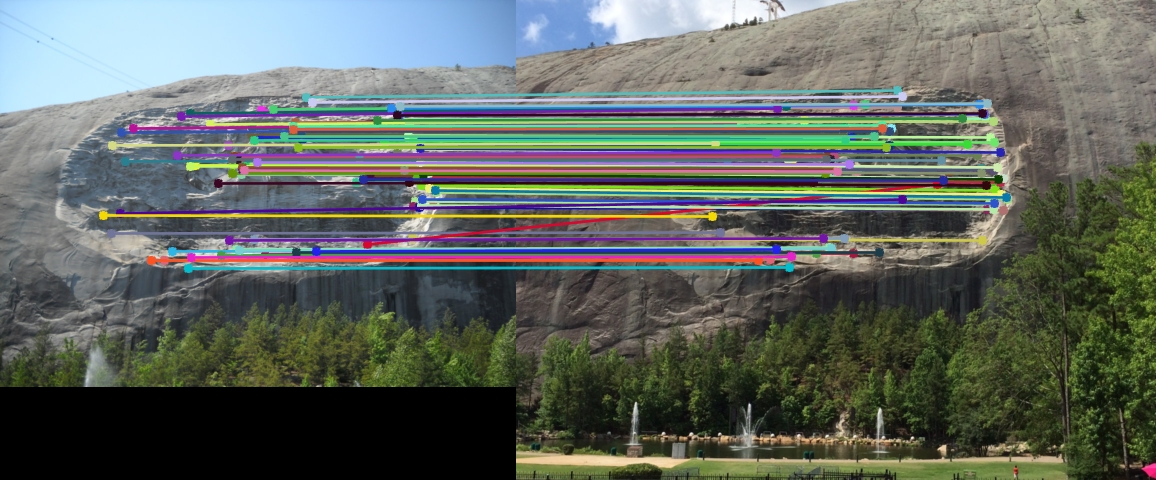
Stone mountain arrows (No evaluation, but appears to be very accurate).