Li Yi

Detection

To identify corners, we apply a small window which shifts to all direction and check if there's a large change in intensity. To do so, we need to compute the change using Harris corner detector:

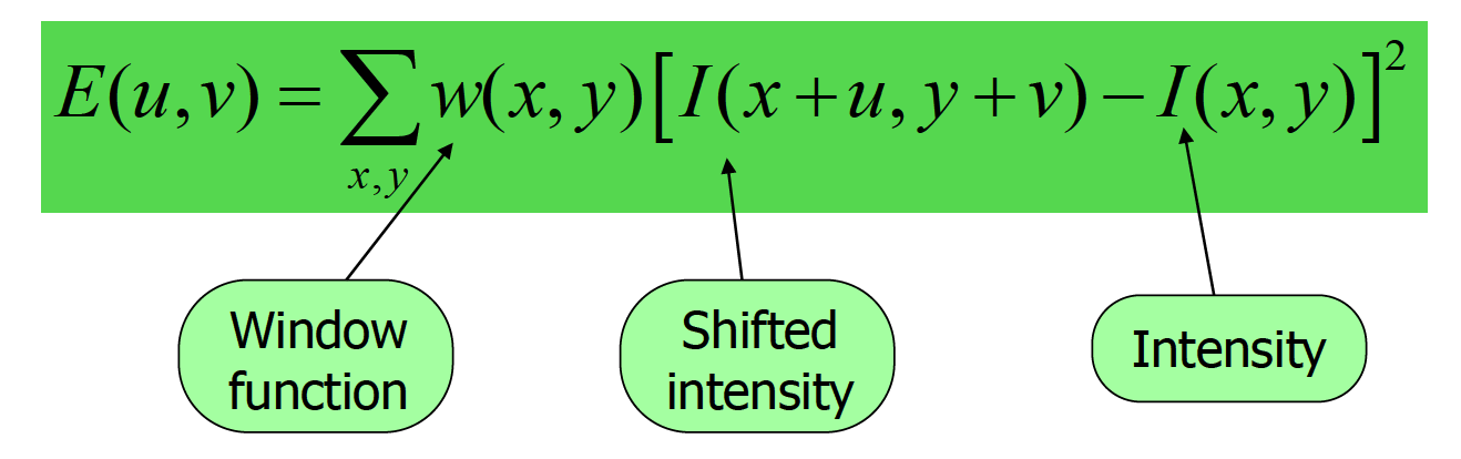
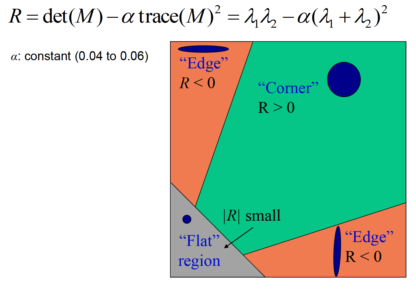
After transformation, eventually we compute a score using two eigenvalues of the matrix. If both eigenvalues are large or score is positive, we know that E increases in all directions so that the point is at corner.

    % Compute Ix, Iy and matrix M to get the corner response function
    [Ix, Iy] = gradient(image);

    filter = fspecial('gaussian', feature_width, sigma);

    M1 = conv2(Ix.^2, filter, 'same');
    M2 = conv2(Iy.^2, filter, 'same');
    M3 = conv2(Ix.*Iy, filter, 'same');

    Det = M1.*M2 - M3.^2;
    Trace = M1 + M2;
    R = Det - alpha * Trace.^2;

    

To avoid that points with high R value are clustered at certain area, we slide image by a 5*5 window and get the maximum value of each section. Also, to avoid that we count in a point of flat region which would result in a comparatively small absolute value of R, we set a threshold as 0.05 of the mean of all R values, to only keep points with sharp changes.

        % Get the maximum of each 5*5 window
        maximum = colfilt(R,[5,5], 'sliding', @max);
        max_final = R.*((R == maximum) & (R>(mean2(R)*0.05)));
        [x,y,confidence] = find(max_final);
    

Finally, since we will compute the descriptor of each point using a 16*16 window to include all the pixels around, we need to filter out those corner points on the edge of image.

        % Remove points near the edge of image
        I = intersect(find(x>feature_width/2 & x<(size(image,1)-feature_width/2)),
        find(y>feature_width/2 & y<(size(image,2)-feature_width/2)));
    

Description

For each of the intereset point, we apply the SIFT vector formation which consists of 8 orientations and 4*4 array of gradient orientation histogram weighted by magnitude. So in total, the descriptor is of 128 dimension.

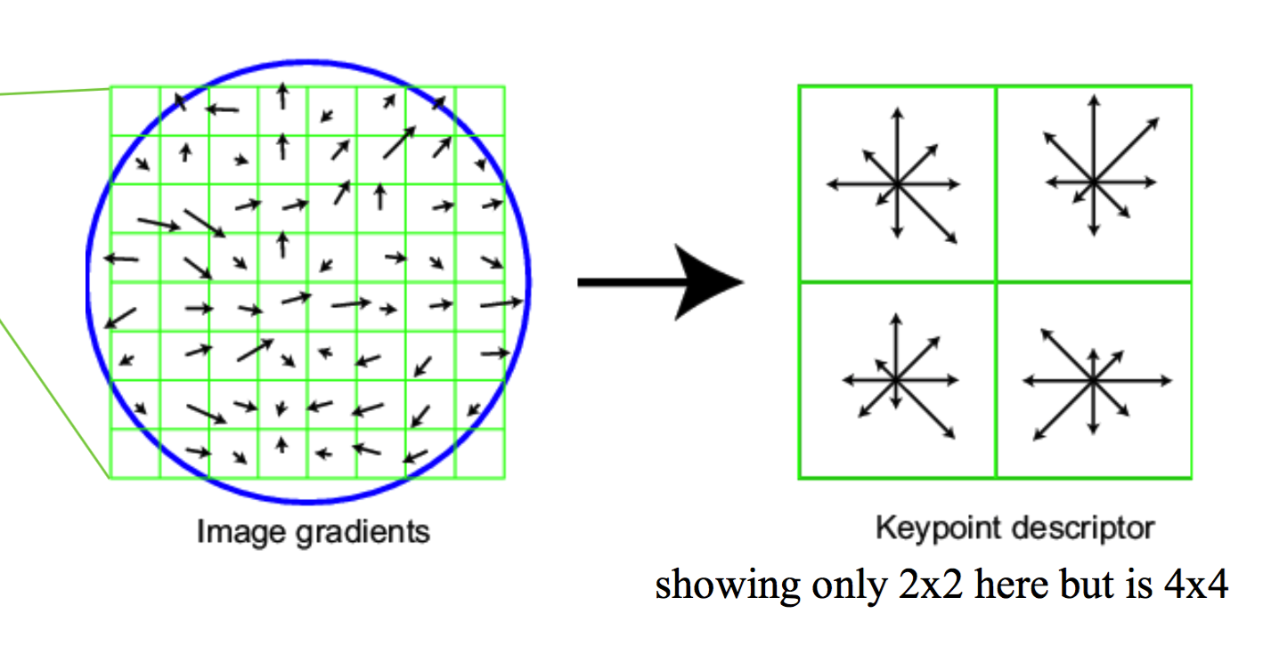
To do so, we first initialize a feature vector with 128 columns and rows as the number of given interest points. Then we loop through each point, set a 16*16 window with the point as the center; evenly divide the window as 4*4, in each section compute the gradient and orientation of all the cells and accumulately add them to the 8 orientation.

        % Compute descriptor of each section in 4*4 window
        descriptor = zeros(1, 8);
        for p = left:(left + feature_width/4 - 1)
            for q = down:(down + feature_width/4 - 1)
                o1 = floor(orien(p, q)) + 1;
                o2 = mod(ceil(orien(p, q)), 8) + 1;
                descriptor(o1) = descriptor(o1) + smooth(p - origin_left + 1, q - origin_down + 1)*
                    (ceil(orien(p, q)) - orien(p, q));
                descriptor(o2) = descriptor(o2) + smooth(p - origin_left + 1, q - origin_down + 1)*
                    (orien(p, q) - floor(orien(p, q)));
            end
        end
    

Finally, to avoid excessive influence of high gradients, we normalize the vector and threshold gradient magnitudes as clamp gradients > 0.2

        % Normalize vector; set threshold and re-normalize
        features(i,:) =  features(i,:) / norm(features(i,:));
        features(i, features(i,:)>0.2) = 0.2;
        features(i,:) =  features(i,:) / norm(features(i,:));
    

Match Points

The simplest approach of matching is to pick the nearest neighbor of each descriptor in vector space. Meanwhile, we compute the distance ratio as NN1/NN2, where NN1 = the distance to the first nearest neighbor and NN2 = the distance to the second nearest neighbor. This ratio represents how confident we are to match two points.

        % Compute distance between pair of point
        D = pdist2(features1, features2);
        for i=1:size(features1, 1)
            [sorted_distance, I]= sort(D(i,:), 'ascend');
            confidences(i) = sorted_distance(1) / sorted_distance(2);
            matches(i, 1) = i;
            matches(i, 2) = I(1);
        end
    

K-d Tree and PCA

The KDTreeSearcher of MATLAB model objects store results of a nearest neighbors search using the Kd-tree algorithm, which speeds up matching process. But k-d tree is generally used by low dimension vector, we need to apply Principal Component Analysis to reduce dimension from 128 to 32.

        % Concatenate features1 and features2
        cat = [features1; features2];
        [coeff, score] = pca(cat);
        reduced_features1 = score(1:size(features1, 1), 1:32);
        reduced_features2 = score((size(features1, 1) + 1):size(cat, 1), 1:32);
    

After reducing dimension to 32, we generate a k-d tree and use minkowski distance to compute the nearest neighbor.

        Mdl = createns(reduced_features2,'NSMethod','kdtree','Distance','minkowski');
        for j = 1:size(reduced_features1, 1)
            Q = reduced_features1(j,:);
            [IdxNN,D] = knnsearch(Mdl, Q, 'K', 2);
            matches(j, 1) = j;
            matches(j, 2) = IdxNN(1);
            confidences(j) = D(1)/D(2);
        end
    

Results in a table

Below are the result of matching between 1) Notre Dame image pair; 2) Mount Rushmore image pair; and 3) Episcopal Gaudi image pair.

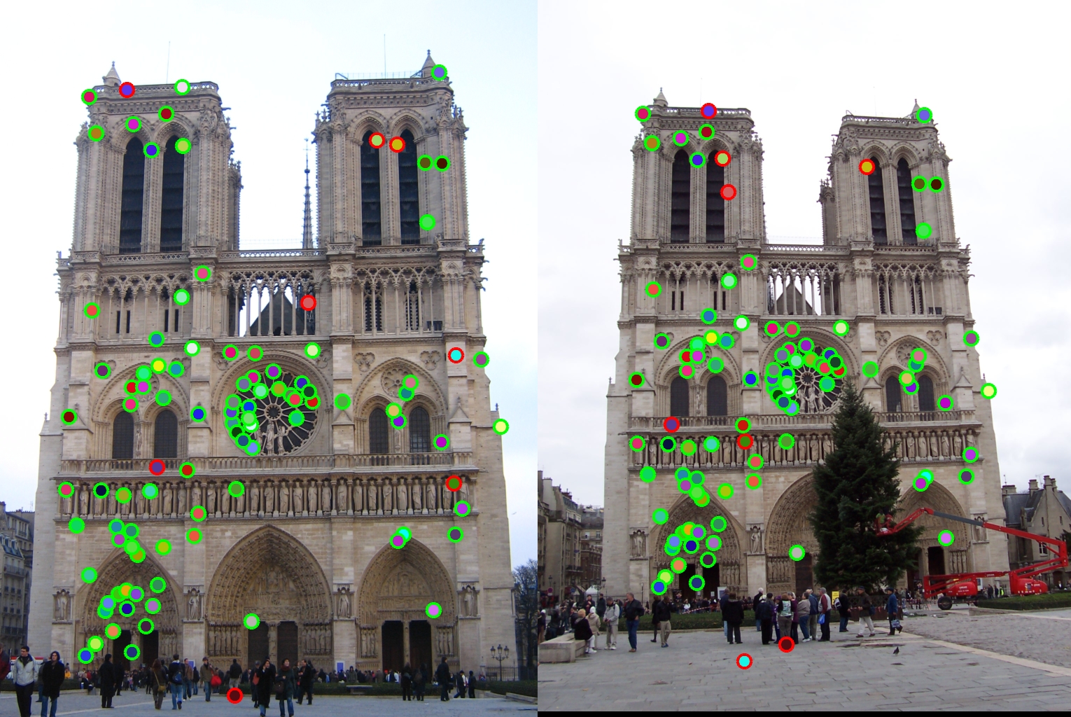
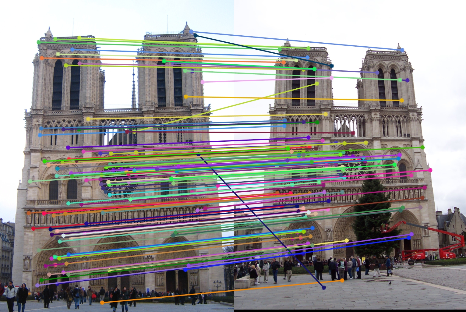
92 total good matches, 8 total bad matches. 92.00% accuracy.

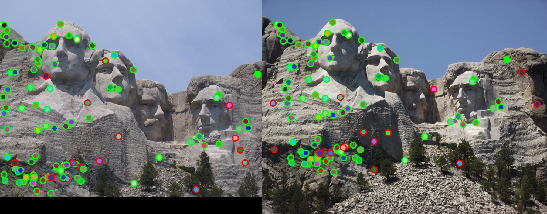
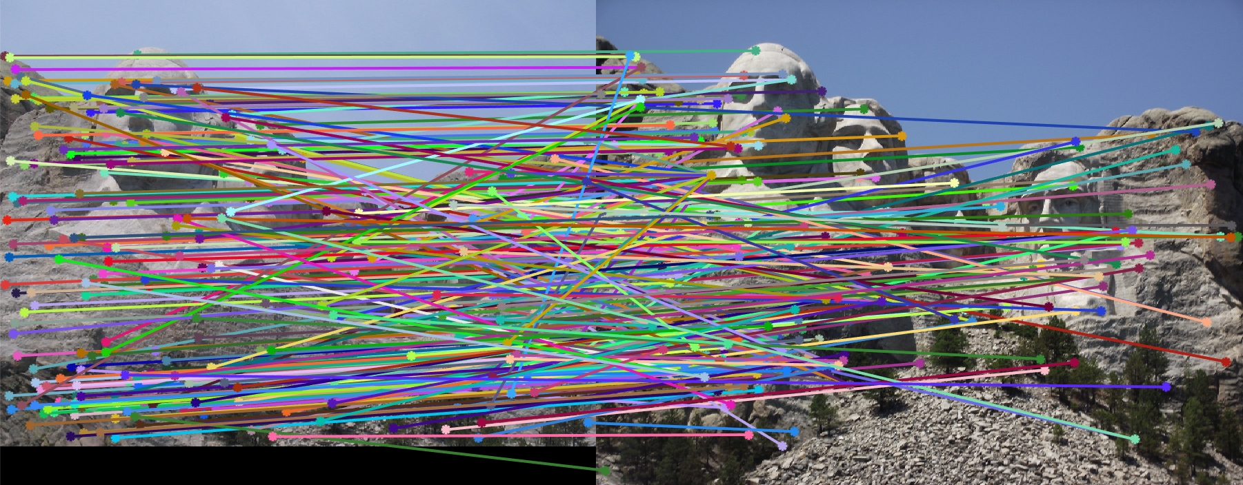
85 total good matches, 15 total bad matches. 85.00% accuracy.

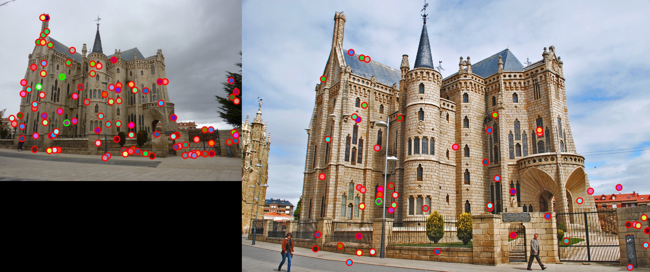
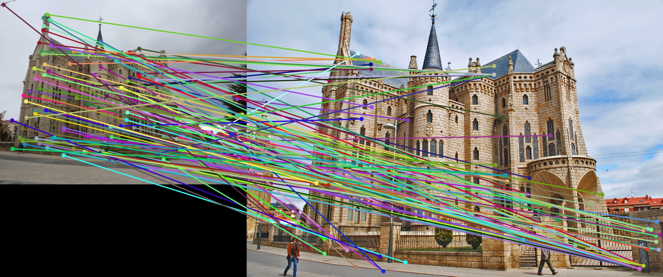
3 total good matches, 97 total bad matches. 3.00% accuracy.