Project 2: Local Feature Matching
Intro
In this project, I implemented a simple version of the SIFT pipeline, which is a process for feature matching between images. The pipeline has several stages. These stages are interest point detection, local feature description, and feature matching. My implementation of each of these stages is described below.
Interest Point Detection
I implemented the Harris corner detector to find around a thousand interest points for each image. Corner detection was implemented in these steps:
- Blur the image with a small gaussian filter.
- Find the x and y derivatives of the blurred image.
- Square the derivatives (elementwise).
- Blur the squared derivatives with a larger gaussian.
- Compute a matrix of interest measures for each pixel (higher is better).
- Find local maxima above a certain interest value threshold and return them as detected feature point locations. Do this by thresholding the interest measure matrix to black and white and then finding local maxima corresponding to connected components.
[i_x, i_y] = imgradientxy(blurred_image);
alpha = .06;
cornerness_matrix = gi_x2 .* gi_y2 - (imfilter(i_x .* i_y, guassian_filter2)).^2 - alpha * ((gi_x2 + gi_y2).^2);threshold = .0005;
thresholded_cornerness_matrix = cornerness_matrix;
thresholded_cornerness_matrix(thresholded_cornerness_matrix=threshold) = 1;
connected_components = bwlabel(thresholded_cornerness_matrix);
% --snip-- correlate maxima to connected components
Local Feature Description
Each feature descriptor was composed of several histograms corresponding to smaller 4x4 areas within the area covered by the descriptor. Each 4x4 area had its own histogram with 8 bins, each bin representing an angle. For each pixel in the 4x4 area, the angle of the overall gradient of that pixel was computed and the bin whose angle was closest to that angle was incremented. The overall gradient of each pixel was computed by using edge filters to find horizontal and vertical edges and then applying atan2 using the horizontal and vertical values as parameters.
horizontal_edges = imfilter(image, [-1 0 1].');

vertical_edges = imfilter(image, [-1 0 1]);
tangents = atan2(horizontal_edges, vertical_edges);
% --snip-- populate histograms
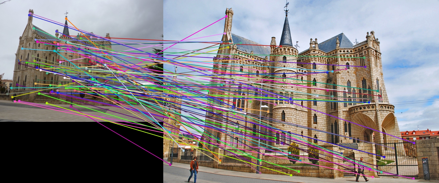
Feature Matching
Feature matching was done using matlab's norm function to judge which pairs of features were closest. A feature could be paired with at most 1 other feature.
Results
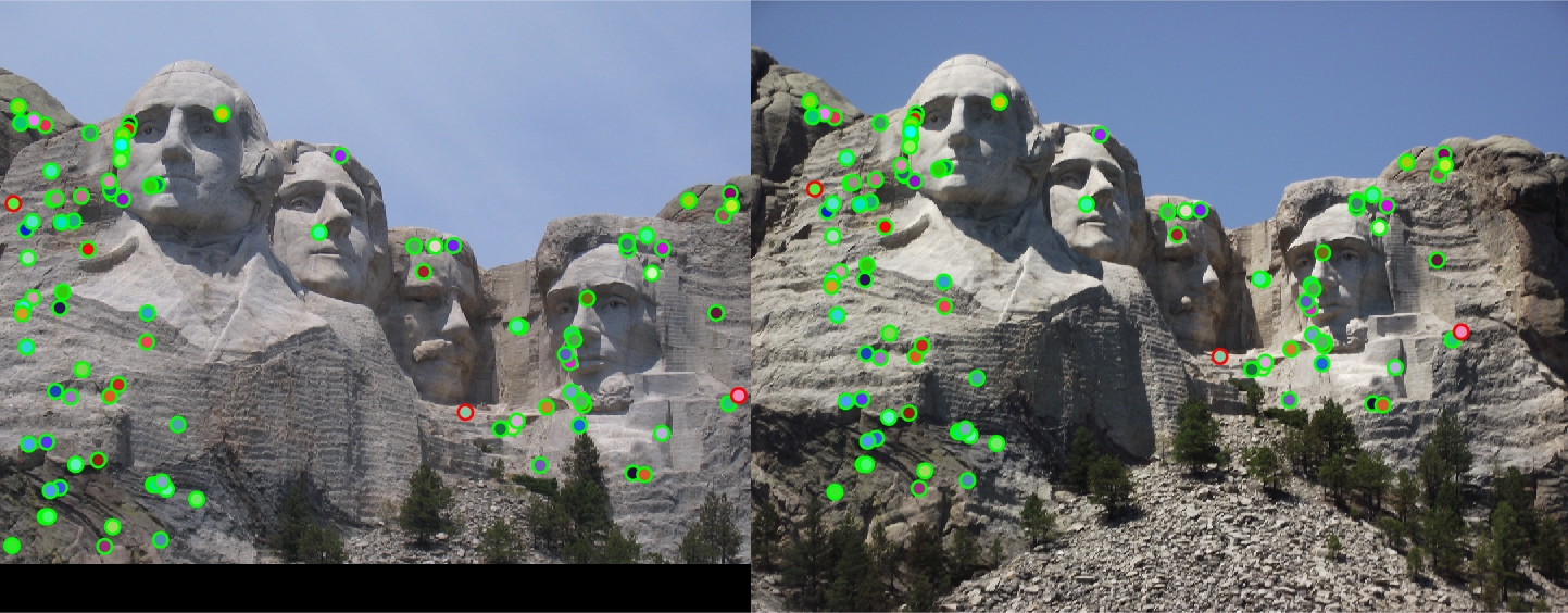
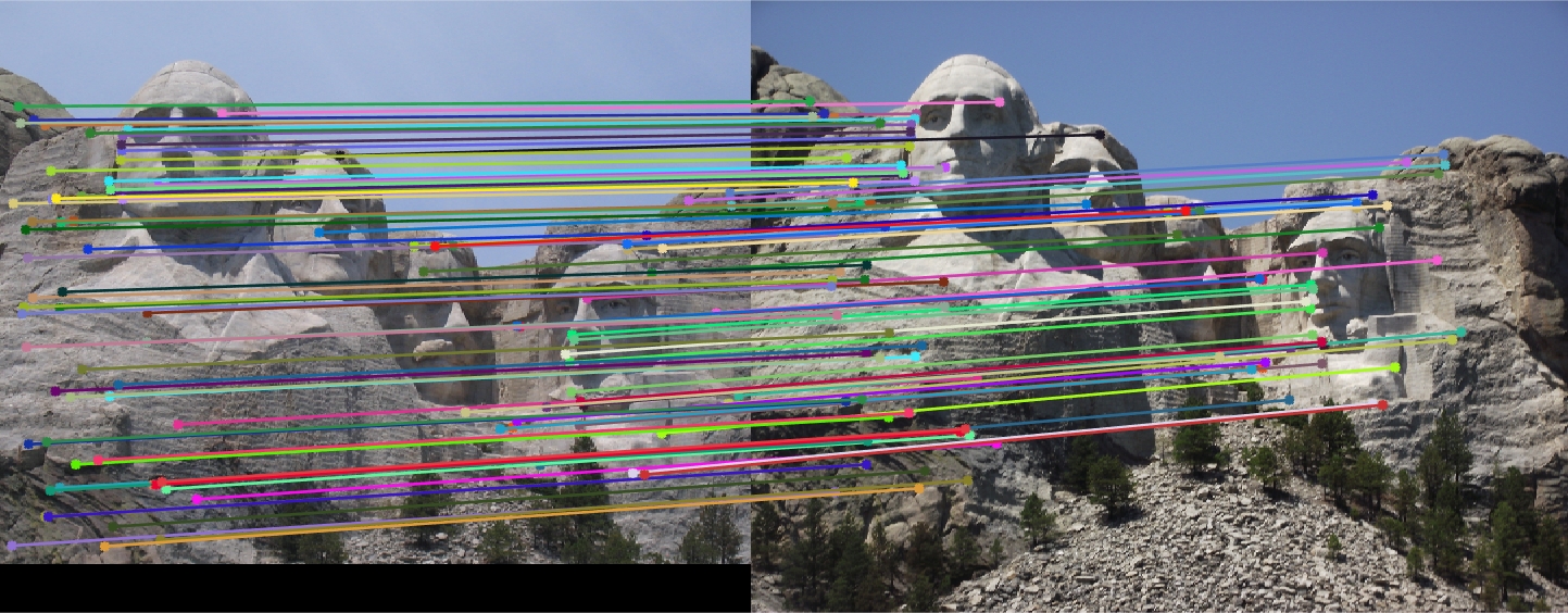
The best results were on the Mount Rushmore pair. I achieved an accuracy of 97% on that image pair.
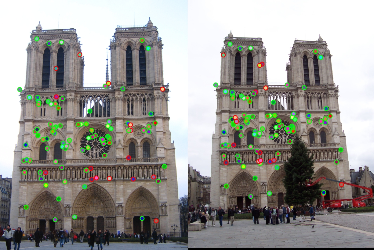
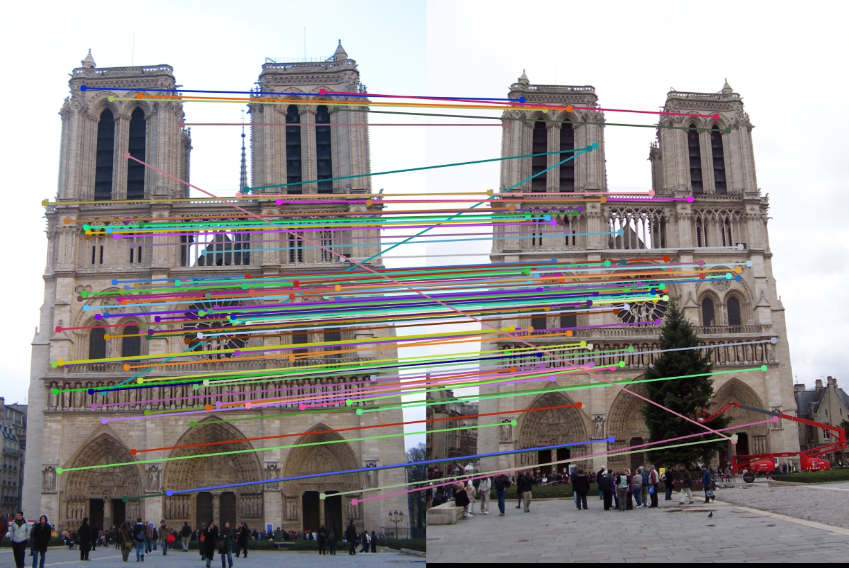
The Notre Dame image pair had the next-best results. I achieved an accuracy of 84% on that image pair.
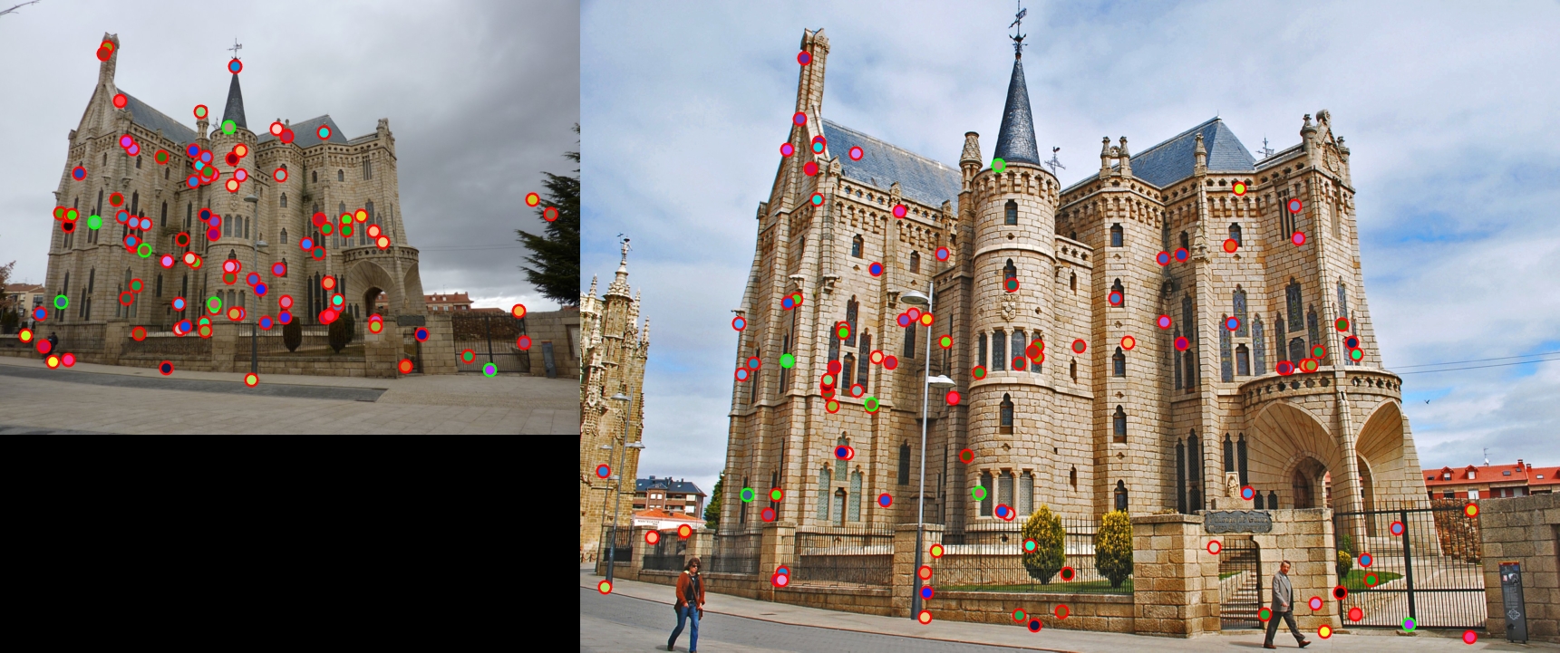
There were several parameters which I had to tweak to achieve these results, especially in the interest point detection algorithm. I settled on a square gaussian of size 5 with sigma .5 for my initial small blur on each of the images. I used a gaussian of size 15 with sigma .5 for my larger blur in step 3 of the algorithm. For alpha, .06 gave the best results along with a certainty threshold of .0005 for constructing the black and white version of the certainty matrix for use with connected components.