Project 2: Local Feature Matching
Overview
For this project, a local feature matching algorithm was implemented to determine if two unique images are "the same" as classified by a human. The algorithm can be broken up into three distinct steps:
This basic implementation was able to successfully find 84% matching features in the simplest of image pairs, and performed moderately well on the medium difficulty image pairs.
Interest Point Detection
To detect interest points, the Harris corner detector was implemented (get_interest_points.m). The following steps are used to implement the corner detector:
Local Feature Detection (simplified SIFT algorithm)
This function (get_features.m) takes in the interest points from the Harris corner detector implementation, and calculates a 128 dimension feature descriptor describing the local behavior at each interest point. The SIFT algorithm chose 128 dimensions as a balance between flexibility and overspecification: lower dimension descriptors perform poorly with changes in lighting, while higher dimension descriptors can become to specified.
The first step in the SIFT algorithm is to detect interest points, or keypoints. A basic Gaussian is convolved with the gradients of the image. Next, the orientation at each keypoint is calculated, along with the gradient magnitude of each keypoint. The code for this step is shown below:
octants = @(x,y) (ceil(atan2(y,x)/(pi/4)) + 4);
[row,col] = size(gx);
orients = zeros(row,col);
for i = 1:row
    for j = 1:col
        orients(i,j) = octants(gx(i,j), gy(i,j));
    end
end
mag = hypot(gx, gy);
Next, each feature is found based off of these keypoints and teir orientations. This part is where the 128 dimension feature descriptor is calculated. Subregions of the image are convolved with a new Gaussian with a sigma equal to half of the feature width. Then, the subregions are collapsed to obtain the 128 dimensions.
gaussianKey = fspecial('Gaussian', [feature_width feature_width], feature_width/2);
c = feature_width/4;
for i = 1:r
    %Weight magnitudes with Gaussian, sigma = 1/2 feature width
    xInd = (x(i) - 2*c): (x(i) + 2*c-1);
    yInd = (y(i) - 2*c): (y(i) + 2*c-1);
    fMag = mag(yInd, xInd).*gaussianKey;
    fOrients = orients(yInd, xInd);

    % Looping through each cell in the frame
    for xx = 0:3
        for yy = 0:3
            cOrients = fOrients(xx*4+1:xx*4+4, yy*4+1:yy*4+4);
            cMag = fMag(xx*4+1:xx*4+4, yy*4+1:yy*4+4);
            for k = 1:8
                val = sum(sum(cMag(cOrients==k)));
                features(i,(xx*32 + yy*8)+k) = val;
            end
        end
    end
end
Finally, the dimensions are normalized to a unit length.
Feature Matching
The final step was to match all interest points, and eliminate any spurious matches (match_features.m). To match interest points, the distance between all points was calculated, then the ratio of the nearest two neighbors to each point is calculated. This nearest-neighbor distance ratio (NNDR) test does a reasonable job of differentiating good matches from bad matches, thus reducing the number of false positives. The basic code to calculate the ratio can be seen below:
r = length(features1(:,1));
c = length(features2(:,1));
distances = zeros(r, 2);
distCalc = @(f1,f2,i,j) sqrt(-dot(f2(j,:)-f1(i,:),f1(i,:)-f2(j,:)));

%O(MN) Complexity
for i = 1:r
    for j = 1:c
        distances(i,j) = distCalc(features1, features2, i, j);
    end
end

[distances, ind] = sort(distances, 2);
confidences = distances(:,2) ./ distances(:,1); %ratio

% Determine which matches are accurate enough to keep
threshold = 1.43;
minConfidenceBound = confidences > threshold;
confidences = confidences(minConfidenceBound);

% Create output matches to be sorted
matches = zeros(size(confidences, 1), 2);
matches(:,1) = find(minConfidenceBound);
matches(:,2) = ind(minConfidenceBound, 1);

% Sort the matches so that the most confident onces are at the top.
[confidences, ind] = sort(confidences, 'descend');
matches = matches(ind,:);
Results
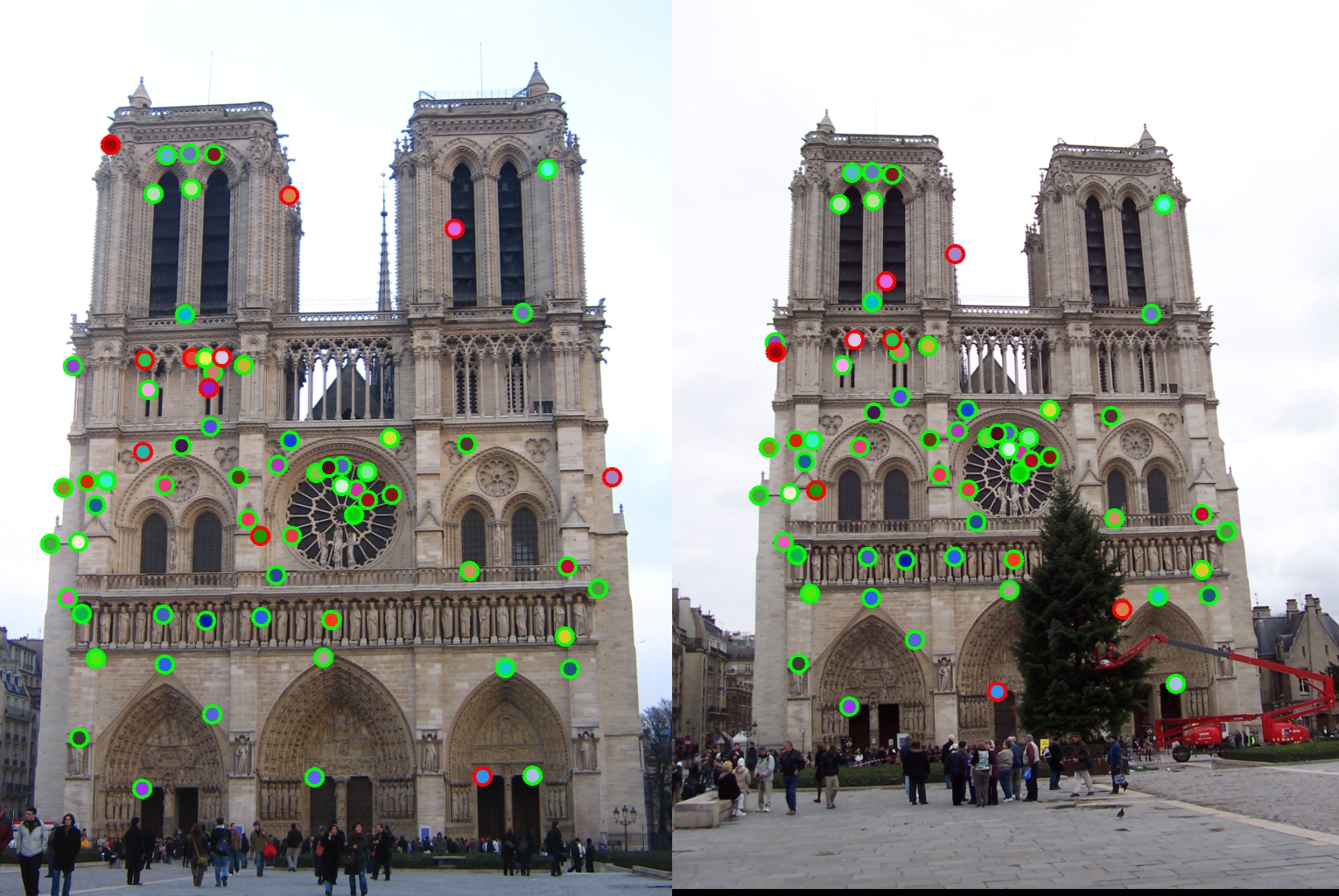
Notre Dame Images: 59 total good matches, 11 total bad matches. 84% accuracy
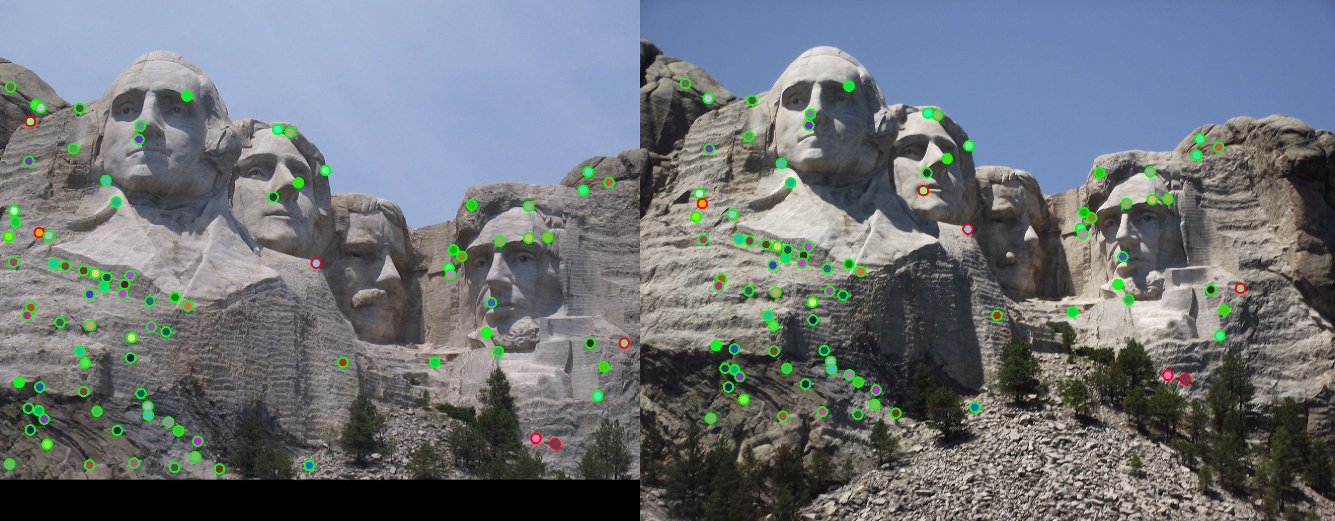
Mount Rushmore Images: 87 total good matches, 6 total bad matches. 94% accuracy
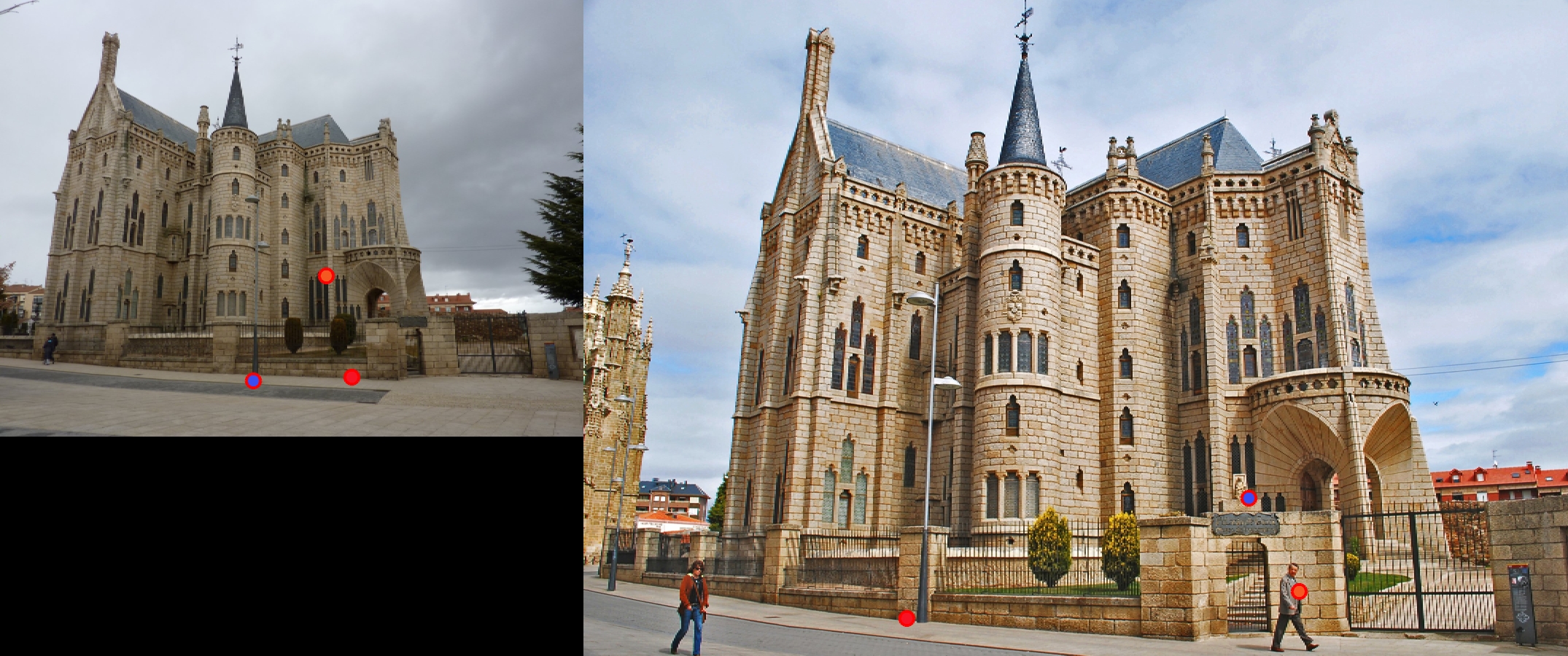
Gaudi Images: 0 total good matches, 3 total bad matches. 0% accuracy. The feature matching threshold was too high for the given image, resulting in an elimination of most interest points.