Project 2: Local Feature Matching
|
The following writeup is organized as follows:
I. Described the match features function
II. Normalized patches as features
III. SIFT-like features
IV. Harris point Detection for Interest points
V. Results of Normalized patches and SIFT-like features
VI. Comparison of paramters
VII. PCA-SIFT like features
VIII. Rotation Invariant SIFT features
IX. Scale and Rotation Invariant features
X. Additional results with SIFT-like features
- Matching Features
- Normalized patches
- SIFT-like features
- Interest Points
I implemented the Harris corner point detection algorithm in the file get_interest_points.m. The steps are described as follows:
1. Used sobel filters to calculate the x and y gradients of the image.
2. Evaluated the cornerness function (Harris corner detection) for each of the pixel and used a threshold to eliminate certian pixels.
3. Perform Non-maximum suppression using a window of size 3x3 on the image to obtain the final interest points for which SIFT-like features are extracted later.
... ... % using sobel filters to find the xgradient and ygradient of the image at % every pixel. sobel1=[-1 0 1; -2 0 2; -1 0 1]; gx=imfilter(image,sobel1); sobel2= sobel1'; gy=imfilter(image,sobel2); gaussian2 = fspecial('gaussian', 3,1); % using a gaussian filter here to smooth the square of the gradients gxy=gx.*gy; gxy=imfilter(gxy, gaussian2); gx2=gx.*gx; gx2=imfilter(gx2, gaussian2); gy2=gy.*gy; gy2=imfilter(gy2, gaussian2); % computing the cornerness function for each point in the image [r,c]=size(image); cornerness=zeros(size(image)); alpha=0.04; for i=1:r for j=1:c m=[gx2(i,j),gxy(i,j); gxy(i,j),gy2(i,j)]; cornerness(i,j)=det(m)-alpha*trace(m)*trace(m); end end % non-maximum suppression - didn't use colfilt() cornerness(cornerness(:)<0.09)=0; ind=find(cornerness(:)>0); for i=1:size(ind,1) % checking if the center is maximum in the window else make it zero if 1<=ind(i)-r-1 && ind(i)-r-1<=r*c && ... 1<=ind(i)+r+1 && ind(i)+r+1<=r*c && ... cornerness(ind(i))>cornerness(ind(i)-r) && ... cornerness(ind(i))>cornerness(ind(i)+r) && ... ... ... else cornerness(ind(i))=0; end end % finding the indices of the final interest points and they are returned ind=find(cornerness(:)>0); ... ...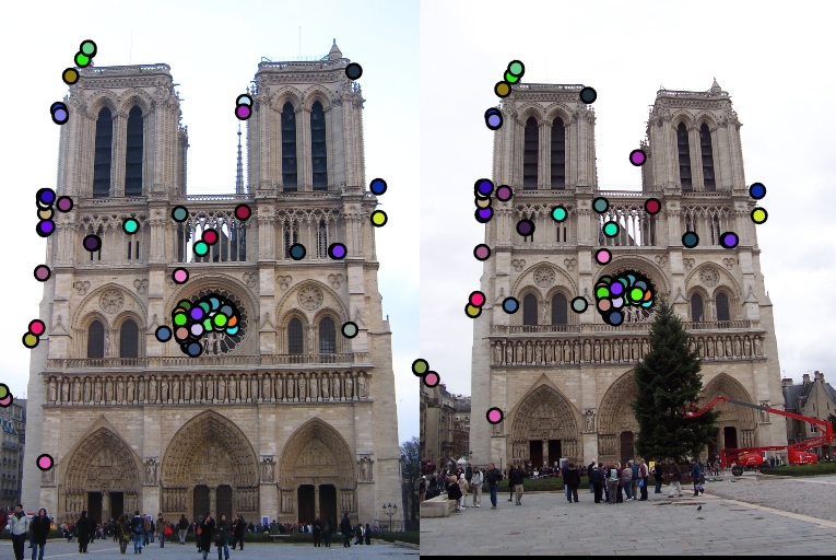
The next two sets of results that follow have been computed using the following parameters:
-> feature_width=16;
-> orientations=8; % number of histrogram bins
-> No clamping of features was done
-> threshold = 0.1; for notre dame
-> threshold = 0.05; for mount rushmore
-> threshold = 0.07; for episcopal gaudi
- Local Feature Matching Results using normalized patches.
- Comparison of various parameters
- PCA SIFT pipeline
- Rotation Invariant SIFT features
- Scale and Rotation Invariant SIFT features
- Additional examples evaluated using SIFT-like features (not invariant and scale versions)
I have implemented match features algorithm in 'match_features.m' as follows:
1. All the euclidean distances between every pair of image features from both the images is calculated.
2. For every image_feature from one of the image, the two nearest neighbors and their distances are retrieved.
3. The image_feature is matched to the nearest feature and their nearest neighbor distance ratio (NN1/NN2) is computed.
4. This nearest neighbor distance ratio is inversely related to the confidence of their matching. So, sorting the matches in ascending order with respect to the nearest neighbor distance ratio will give you matches in the order of confidence. This is the Ratio test.
5. Out of these, the top 100 matches are selected and evaluated further.
		...
		...
		% distance between every pair of image_features from both images is calculated here
		% and the two nearest neighbors and their distances are retrieved
		[D,I] = pdist2(features2, features1,'euclidean','Smallest',2);
		I=I'; D=D';

		% nearest neighbor distance ratio is computed for all the image_features
		% from image1
		listc = D(:,1)./D(:,2);
		threshold=0.8;

		matches=zeros(0,2);
		confidences=zeros(0,1);

		% assigning all the matches to the closest neighbor
		for i=1:size(listc,1)
			%if listc(i)> threshold
			    m=[i I(i,1)];
			    matches=[matches; m];
			    confidences=[confidences; listc(i)];
			%end
		end

		% confidences are inversely related to NN distance ratio.
		% so sorted them in ascending order
		[confidences,ind]=sort(confidences,'ascend');
		matches=matches(ind,:);

		%picking the top 100 matches and their confidence values.
		if size(matches,1)>100
			matches=matches(1:100,:);
			confidences=confidences(1:100);
		end
    		...
    		...
This is written in the 'get_features2.m' file. A 16x16 window is considered around every interest point and these intensities around every interest point are reshaped to form a 256 dimensional descriptor which can be used for matching of interest points. To avoid the case of boundary pixels (if any), the image is padded around with zeros (although this does not make sense when extracting a descriptor from such a window around the interest point with no useful information).
	...
	...
	% padding to avoid index errors when using cheat interest points
	padimage = padarray(image,[(feature_width/2) (feature_width/2)]);
	padimage = padarray(padimage,[(feature_width/2) (feature_width/2)],'post');
	% the intensities in the 16x16 patch around the interest point are obtained
	% and these are then reshaped into a vector to form a 256 dimensional
	% descriptor for that interest point. These descriptors are now sent on
	% matching
	for i=1:length(x)
		local=padimage(x(i):x(i)+(feature_width-1),y(i):y(i)+(feature_width-1));
		local2=reshape(local',size(local,1)*size(local,2),1);
		local2=local2/norm(local2);
		features=[features;local2'];
	end
    	...
    	...
This is available in the 'get_features.m' file. I performed the following steps to obtain SIFT-like features for the given interest points of an image.
1. Calculated the gradient's magnitude and direction using the imgradient function on the image. Also padded the resulting gradient magnitude and direction matrices for the boundary point cases.
2. Considering a window of size 16x16 around the interest point on the image gradients, I divide the window into 4x4 cells each of size 4x4.
3. Now, for each 4x4 cell, a histogram is contsructed with 8 bins with angles (-180,-135,-90,-45,45,90,135) representing each bin. Each pixel contributes to both the closest angle bins of the histrogram based on the closeness to the bin using the gradient magnitude at that pixel. The gradient magnitudes are also downweighted by a Gaussian fall-off function in order to reduce the influence of gradients far from the center, as these are more affected by small misregistrations.
4. Features are constructed for each of the 4x4 cells in the window and appended to form the final feature descriptor for the interest point.
5. The final feature descriptor of the interest point is also normalized to reduce the effects of contrast.
...
...
[gmag,gdir] = imgradient(image);

% padded the gradient direction and magnitude to avoid index errors for
% interest points on the boundary
% padding this image to avoid boundary cases
padgdir = padarray(gdir,[(feature_width/2) (feature_width/2)]);
padgdir = padarray(padgdir,[(feature_width/2) (feature_width/2)],'post');

padgmag = padarray(gmag,[(feature_width/2) (feature_width/2)]);
padgmag = padarray(padgmag,[(feature_width/2) (feature_width/2)],'post');

% 8 orientation bins for the graidient direction histogram
jump=feature_width/4;
orientations=8;
features = zeros(0, orientations*jump*jump);

for i=1:length(x)
    local=padgdir(x(i):x(i)+(feature_width-1),y(i):y(i)+(feature_width-1));
    local2=padgmag(x(i):x(i)+(feature_width-1),y(i):y(i)+(feature_width-1));
    feature=zeros(0,feature_width*jump*jump);
    for j=1:jump:feature_width
        for k=1:jump:feature_width
            subm1=local(j:j+jump-1,k:k+jump-1);
            subm2=gaussian(j:j+jump-1,k:k+jump-1);
            subm3=local2(j:j+jump-1,k:k+jump-1);
            ft=zeros(1,orientations);
            % weigh each pixel's contribution to both the closest bins
            % based on closeness to the angle, also the gradient magnitude
            % and a gaussian filter of size equal to the window
            for m=1:jump
                for n=1:jump
                    if subm1(m,n)>=-180 & subm1(m,n)<-135
                        %ft(1)=ft(1) +
                        ft(1)=ft(1)+(cosd(subm1(m,n)+180))*subm3(m,n)*subm2(m,n);
                        ft(2)=ft(2)+(cosd(-135-subm1(m,n)))*subm3(m,n)*subm2(m,n);

                    elseif subm1(m,n)>=-135 & subm1(m,n)<-90
                        ft(2)=ft(2)+(cosd(subm1(m,n)+135))*subm3(m,n)*subm2(m,n);
                        ft(3)=ft(3)+(cosd(-90-subm1(m,n)))*subm3(m,n)*subm2(m,n);
                    ...
                    ...
                    ...
            feature=[feature, ft];
        end
    end
    % normalizing the feature to reduce the illumination effect.
    feature=feature/norm(feature);
...
...
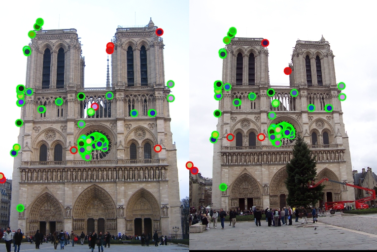
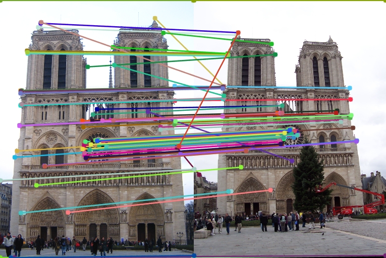
| Interest points | Showing Correspondence | Evaluating the matches | Accuracy |
|
|
|
77% |
|
|
|
44% |
|
|
|
1% |
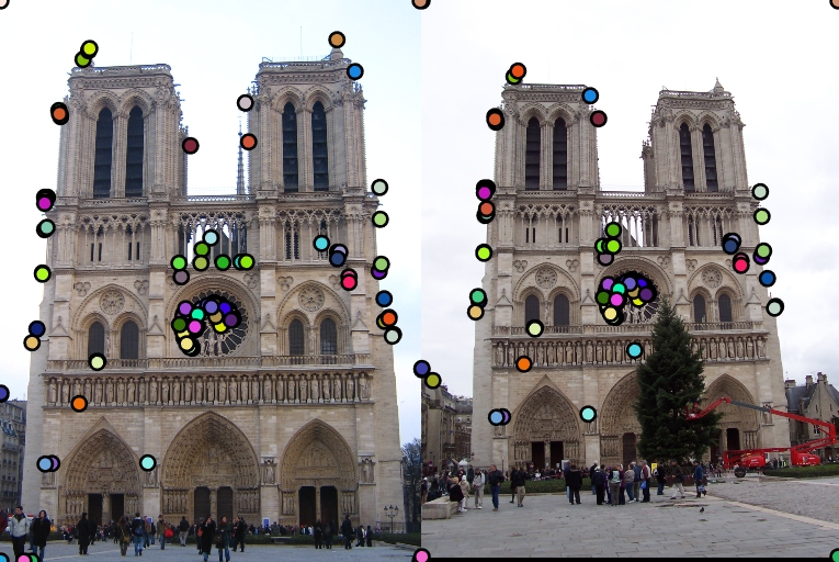
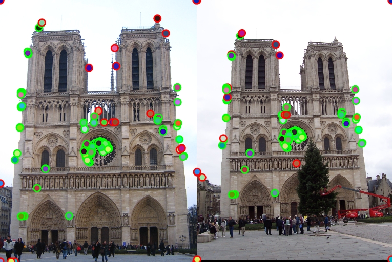
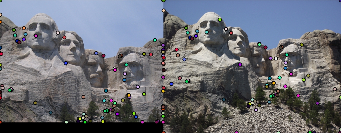
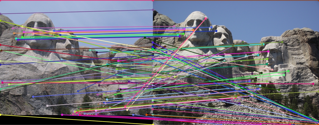
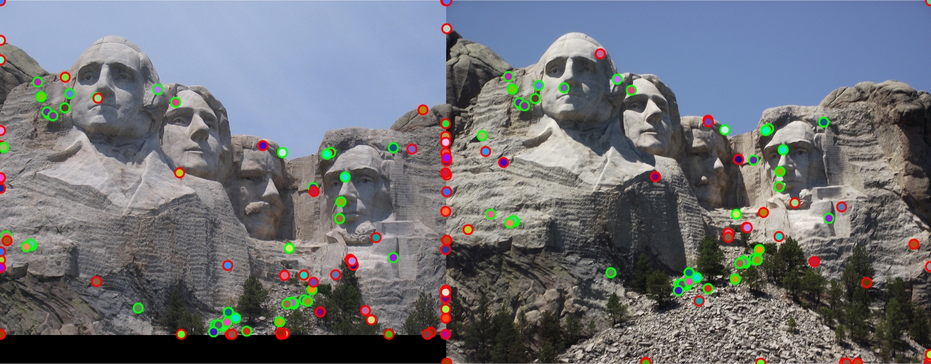
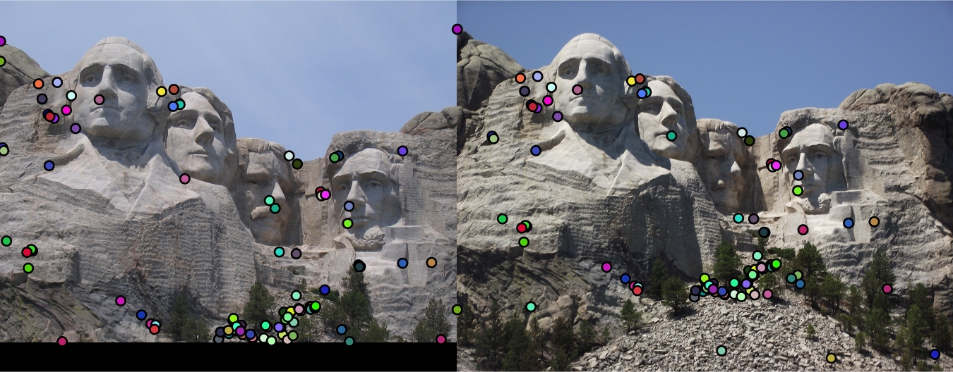
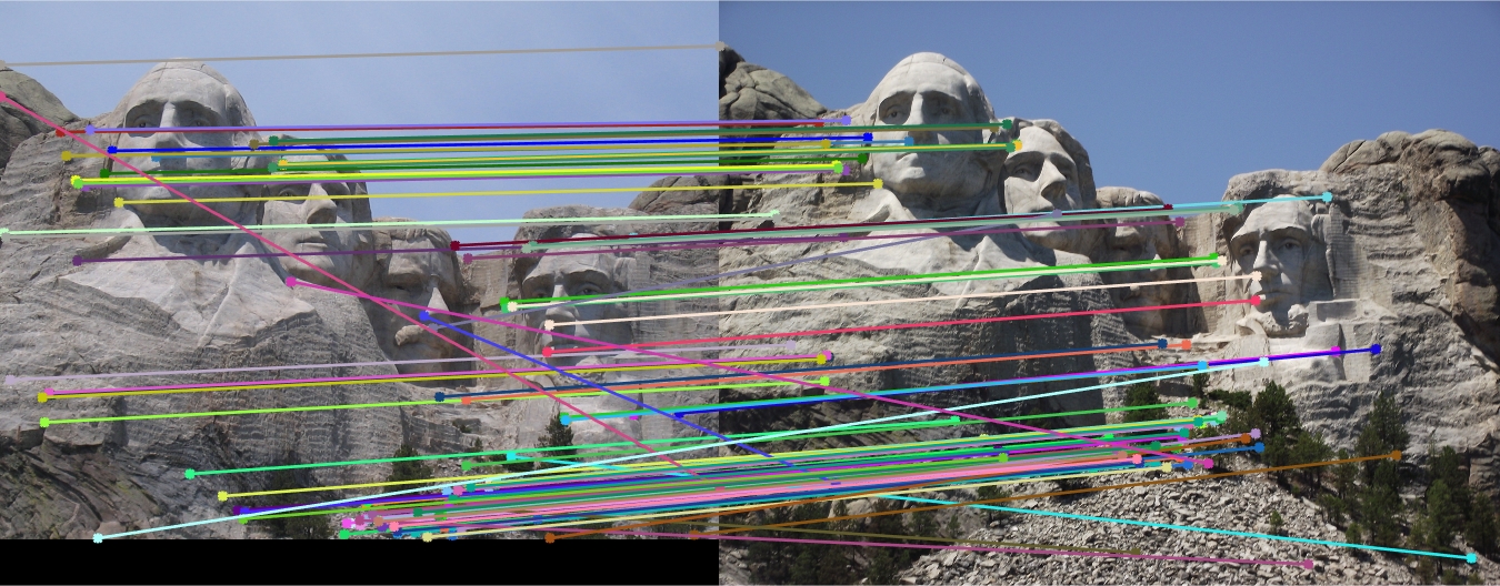
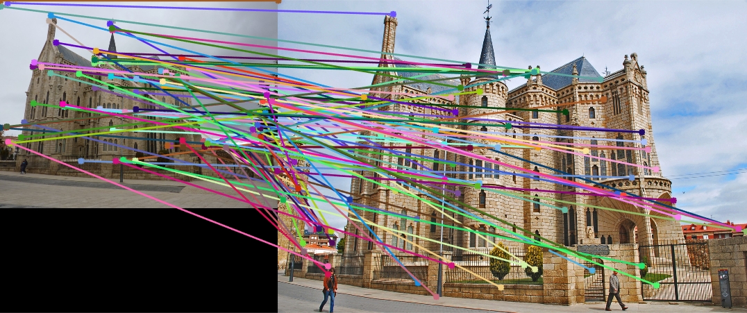
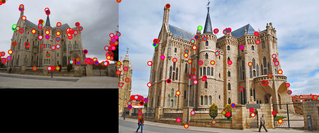
Local Feature Matching Results using the SIFT pipeline described above.
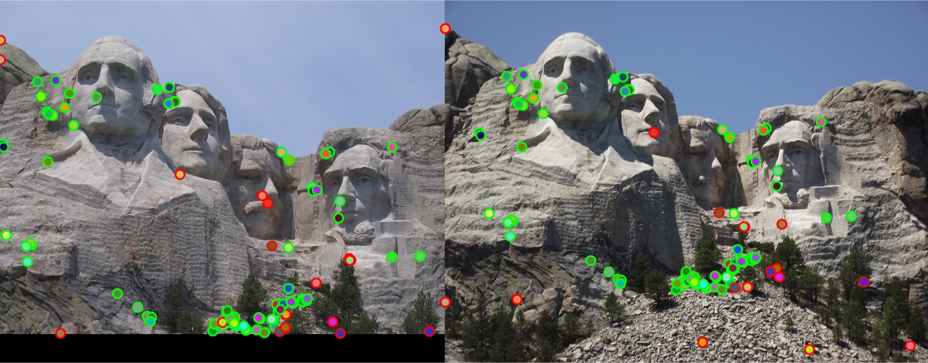
| Interest points | Showing Correspondence | Evaluating the matches | Accuracy |
|
|
|
|
91% |
|
|
|
82% |
|
|
|
4% |
1. I found the accuracies for each of the pair of images to be changing using various thresholds for interest points.
The optimal threshold for each of the pairs is:
-> threshold = 0.1; for notre dame
-> threshold = 0.05; for mount rushmore
-> threshold = 0.07; for episcopal gaudi
The accuracy seems to be decreasing on increasing the threshold for the above pair of images.
2. Also, I found the accuracy to be increasing on normalizing the feature obtained for each interest point in 'get_features.m' file.
I tried to create a lower dimensional descriptor that is still accurate enough. If the descriptor is 32 dimensions instead of 128 then the distance computation should be about 4 times faster. PCA would be a good way to create a low dimensional descriptor. I used 100 random images downloaded from http://lear.inrialpes.fr/~jegou/data.php .
Clearly, It would actually be better if you compute PCA-SIFT features by doing PCA only on the features from the pair of images involved. But then, the SIFT features are not universal, which they are supposed to be. If we change our basis for every image or pair of images, we can no longer compare the SIFT features obtained through such methods across large datasets.
The chosen 100 images are inside the folder 'pca_images' placed in the 'data' folder. The basis computed from the 100 images is saved in 'pca_basis.mat' and this is used to compute the reduced representation of the local descriptors. The actual files used for the computation of the basis are placed in the 'pca_sift' folder.
1. So, I computed the interest points (around 100-150 interest points from each image) from these 100 images and
2. then extracted the SIFT features from those points and images.
3. I then computed the PCA basis on the local descriptors obtained from many images.
4. This set of basis vectors are saved and they are used everytime to compute the reduced representation of the local descriptors for any new image under consideration.
In order to run this PCA-SIFT features, all you need to do is to uncomment the following line in 'proj2.m' file after calling the function get_features().
[image1_features,image2_features]=get_pca_features(image1_features,image2_features);
The results that follow have been computed using the following parameters:
		-> feature_width=16;

		-> orientations=8; 	% number of histrogram bins

		-> No clamping of features was done

		-> threshold = 0.1; for notre dame

		-> threshold = 0.05; for mount rushmore

		-> threshold = 0.07; for episcopal gaudi
| Image used | SIFT-like features | Dimension Size | PCA-SIFT features 1 | Reduced Dimension size 1 | PCA-SIFT features 2 | Reduced Dimension size 2 |
| Notre Dame |
Accuracy: 91% Time taken: 21.24 sec Time for matching: 0.14 sec |
128 |
Accuracy: 83% Time taken: 20.58 sec Time for matching: 0.08 sec |
64 |
Accuracy: 45% Time taken: 26.68 sec Time for matching: 0.05 sec |
32 |
| Mount Rushmore |
Accuracy: 82% Time taken: 40.39 sec Time for matching: 0.014 sec |
128 |
Accuracy: 46% Time taken: 40.43 sec Time for matching: 0.07 sec |
64 |
Accuracy: 13% Time taken: 47.22 sec Time for matching: 0.034 sec |
32 |
| Episcopal Gaudi |
Accuracy: 4% Time taken: 64.23 sec Time for matching: 0.32 sec |
128 |
Accuracy: 2% Time taken: 63.83 sec Time for matching: 0.16 sec |
64 |
Accuracy: 1% Time taken: 67.3 sec Time for matching: 0.09 sec |
32 |
I also tried to build local feature descriptor such that the SIFT-like features obtained are rotation invariant in the 'get_features_rotation.m' . The algorithm that I followed to obtain such features is as follows:
1. Obtain the interest points from the images as mentioned in IV.
2. While extracting the histogram features from the 4x4 cell in the 16x16 window around the interest point, find the dominant direction for that particular cell and rotate that particular cell using the inbult imrotate such that the dominant direction is along the x-axis (i.e. 0 degrees).
3. Now extract the SIFT-like features in the same fashion as described for the rotated cell. Observe that this is done for all the cells in the window and only then the features are extracted for both the images. Hence, even if a cell is rotated in another image it is rotated back to make the dominant direction along the x-axis. This makes the features rotation invariant.
4. Continue matching and rest of the steps as described above.
	...		% get_features_rotation.m file
	... 	% histogram construction on original cell
	[m,index]=max(ft);		% find the dominant direction and rotate the cell such that
    					% the dominant direction aligns along the x-axis (0 degrees)
    	deg=(index-1)*45-180;
    	subm1=imrotate(subm1,deg);
    	subm2=imrotate(subm2,deg);
    	subm3=imrotate(subm3,deg);
   	ft=zeros(1,orientations);
	...		% histogram construction on the rotated cell
	...
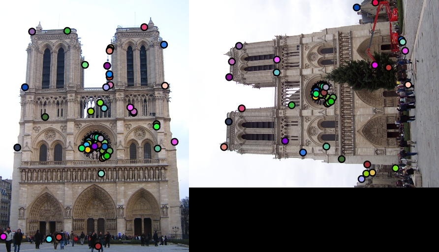
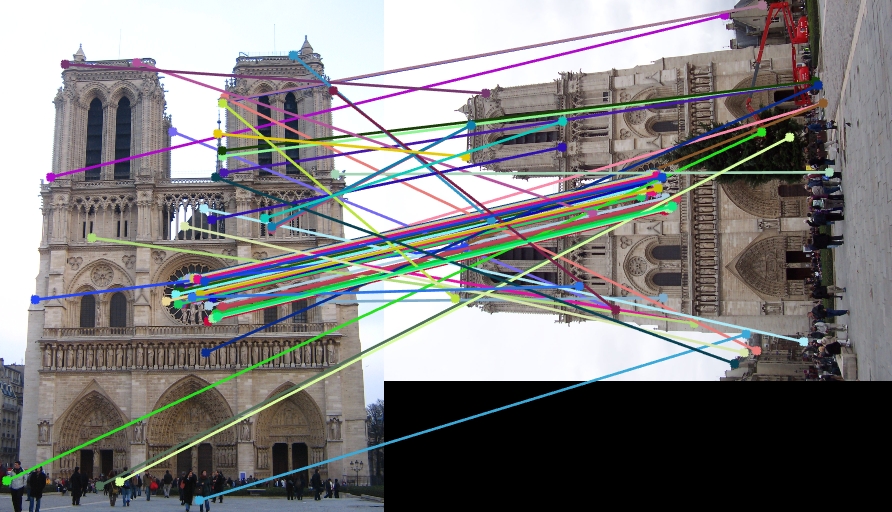
| Interest points | Showing Correspondence |
|
|
|
|
|
|
I have also tried implementing the sift pipeline such that the features would be scale and rotation invariant in the files in the folder 'scale_rot_sift'.
1. I have obtained multiple scales of each image in the pair and obtained interest points independently and
2. then also the local feature descriptors that are rotation invariant independently for each scaled image.
3. Now, all these scaled image1 and scaled image2 are compared with each other to find matches with highest accuracy and their scales are noted.
	...		% get_interest_points_scale.m file
	... 	% run for multiple loops of scales and interest points are obtained at each scale
	for count=1:limit
    		scale_factor=0.9^(count-1);
	...		% similar to extracting interest points as above
	end
	...
	...
	...		% get_interest_points_scale.m file
	... 	% run for multiple loops of scales and rotation invariant features are obtained at each scale
	for count=1:limit
    		scale_factor=0.9^(count-1);
	...		% similar to extracting rotation invariant features as above
	end
	...
	...
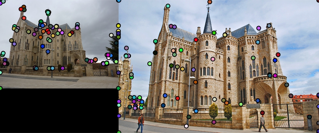
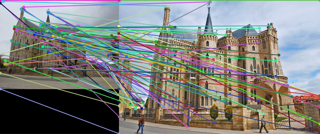
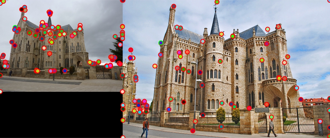
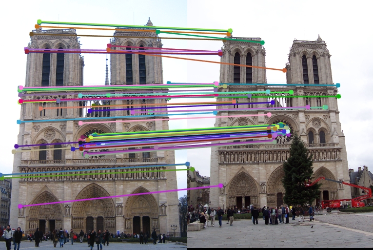
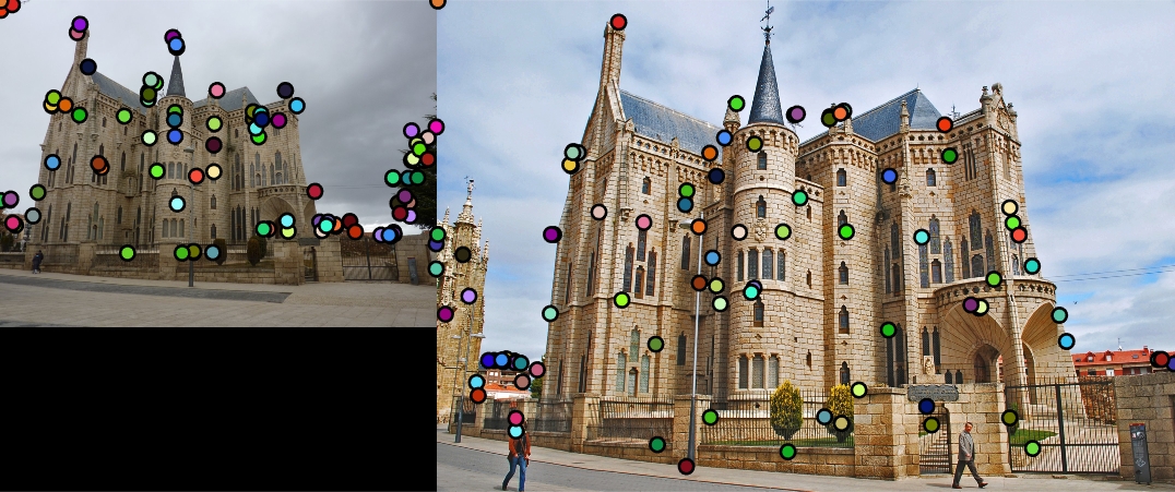
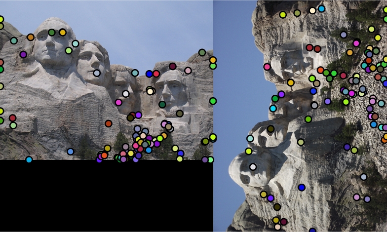
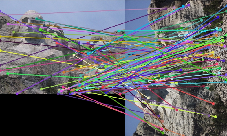
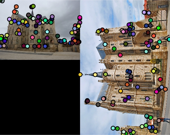
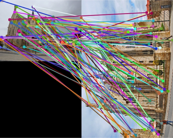
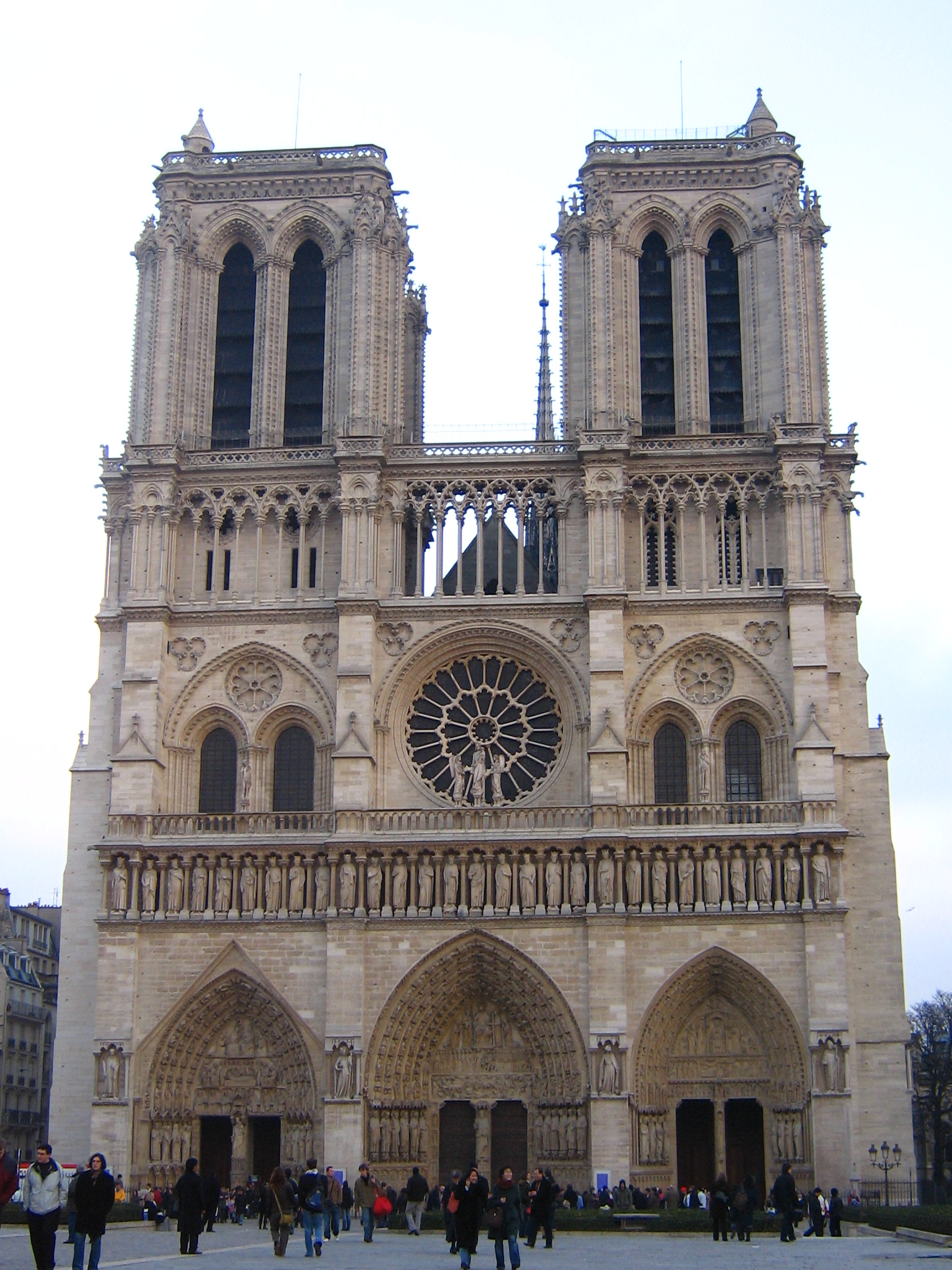
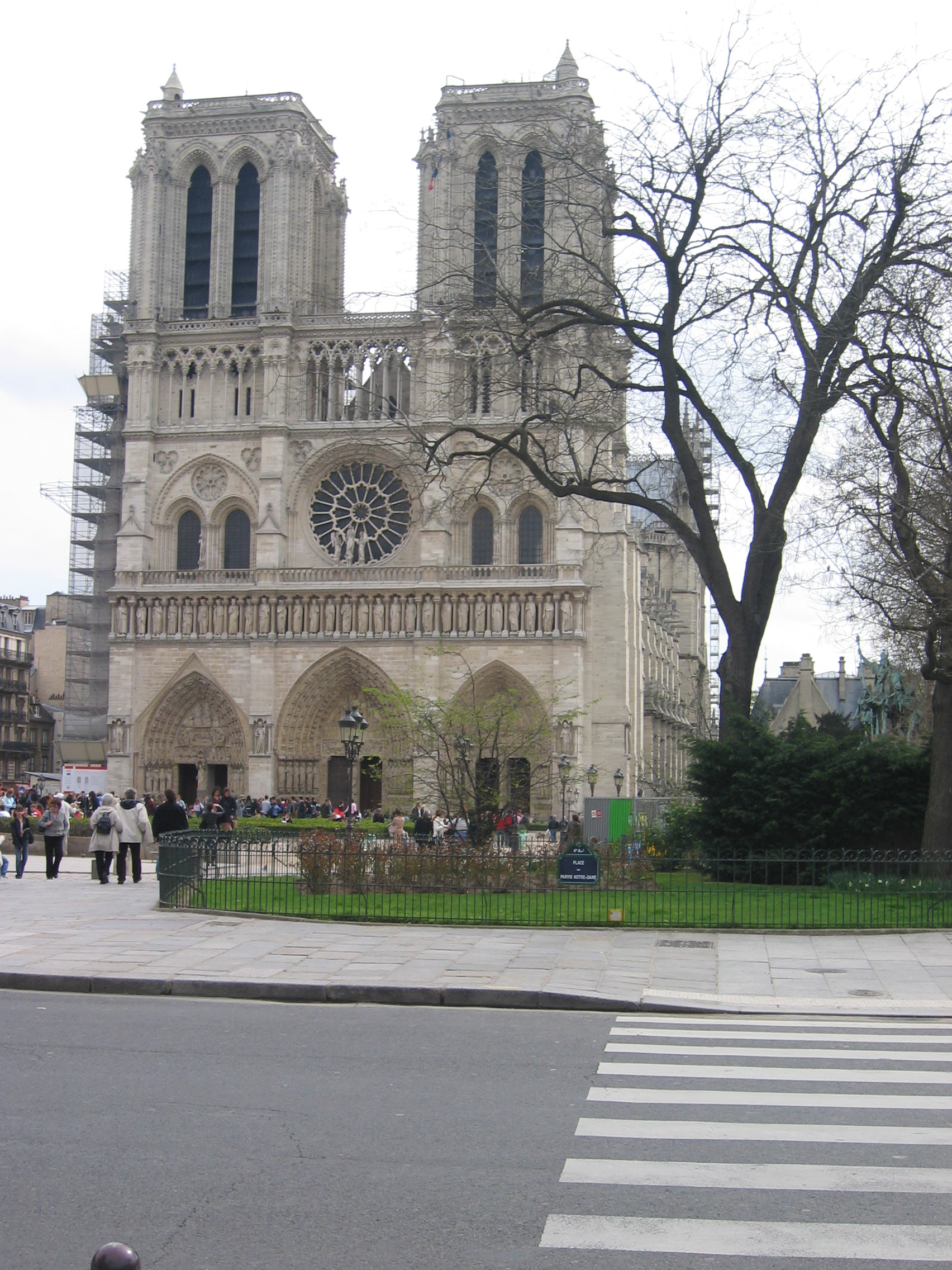
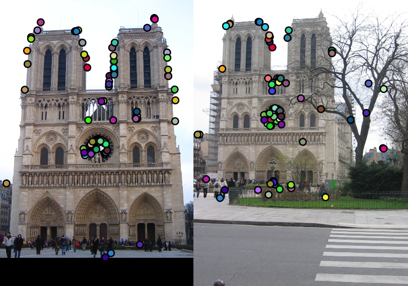
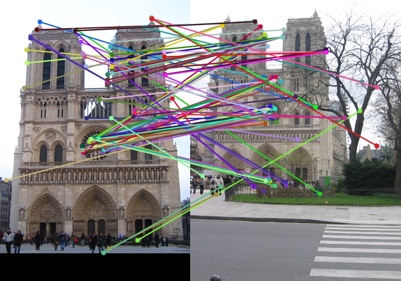
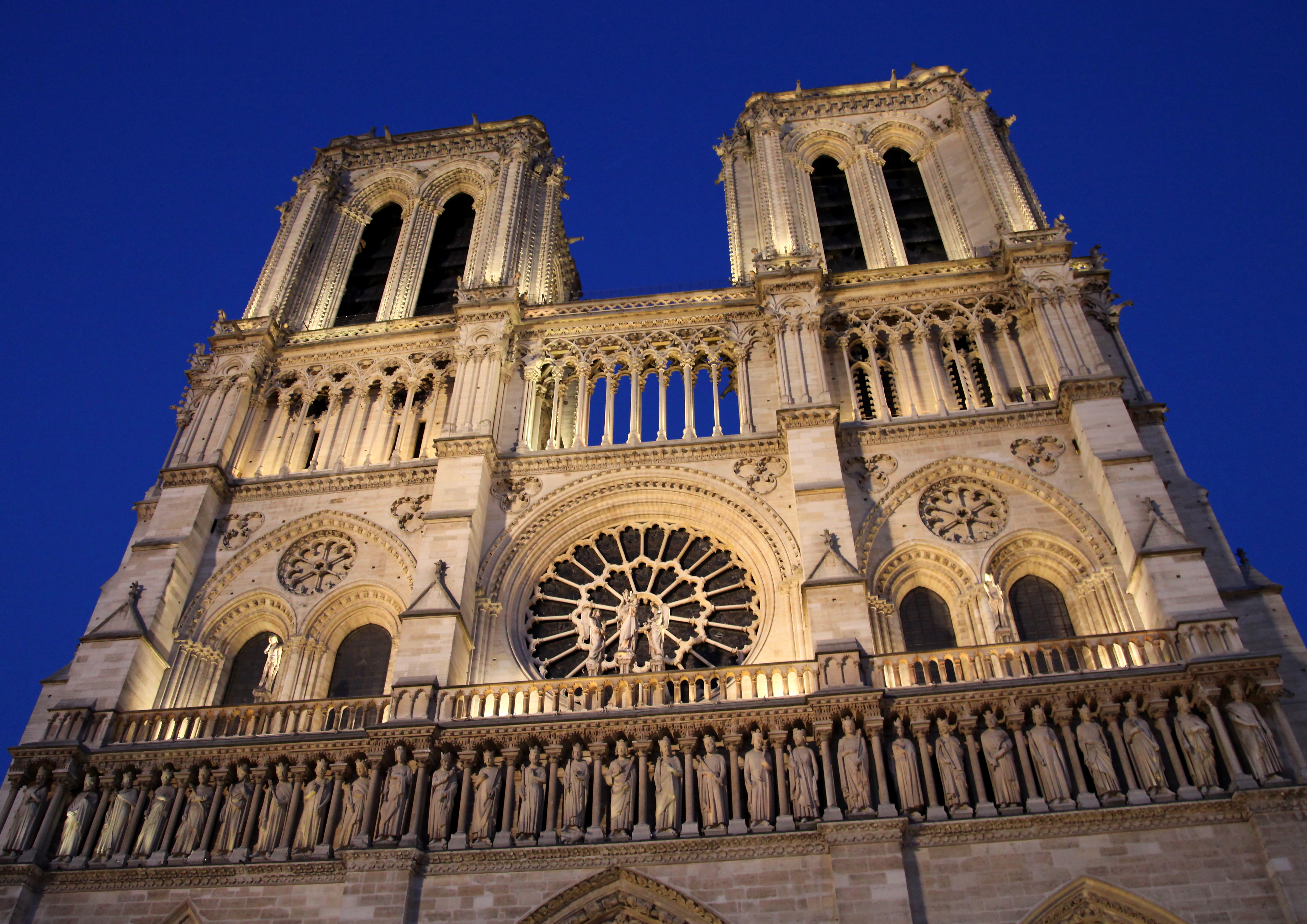
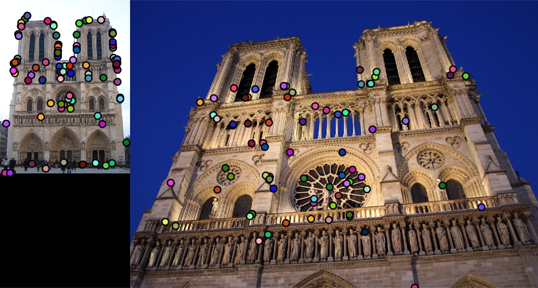
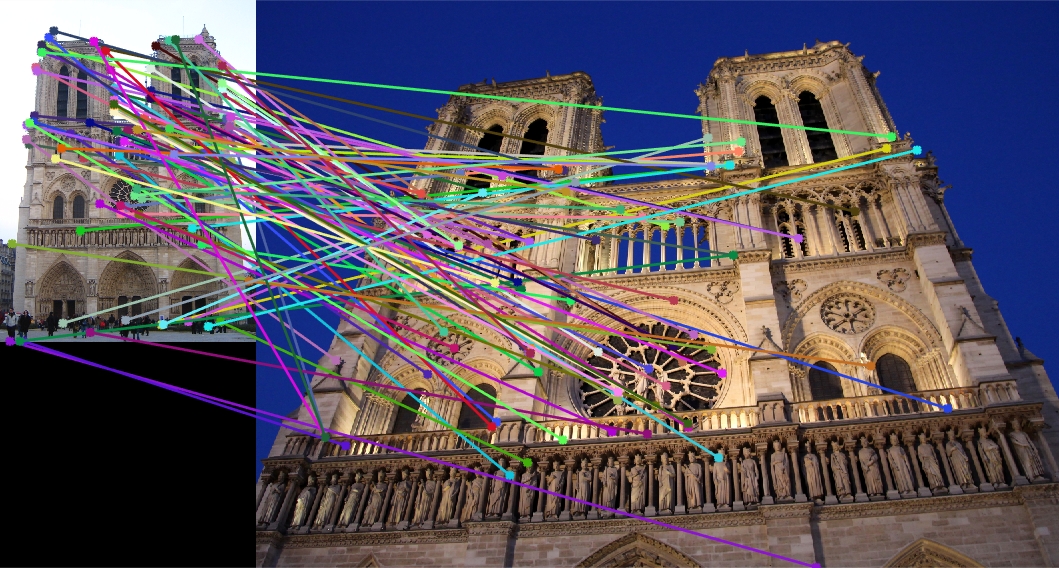
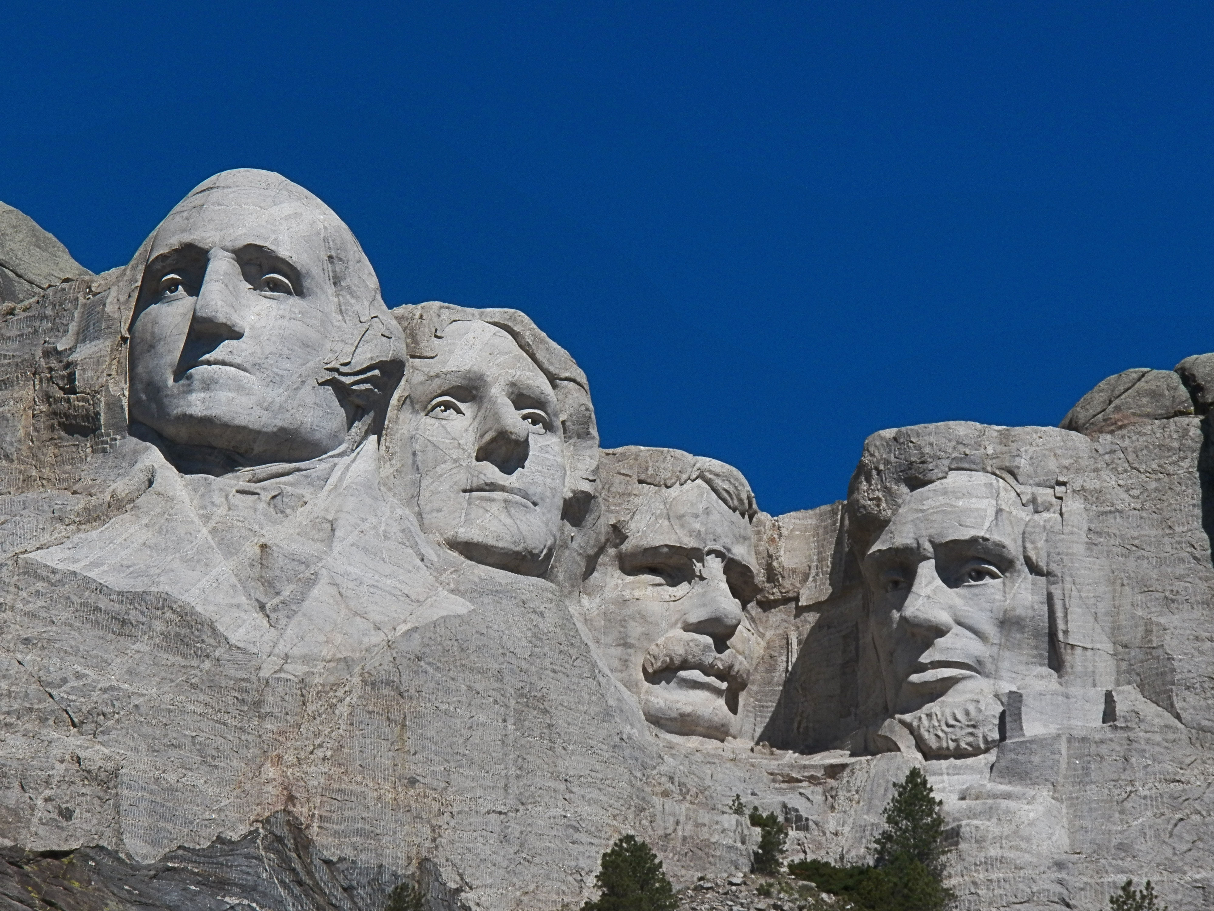
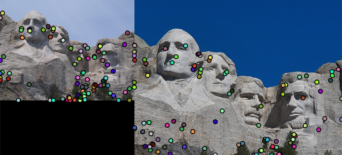
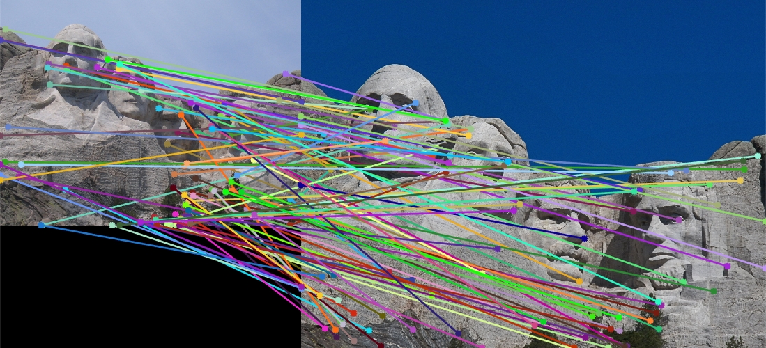
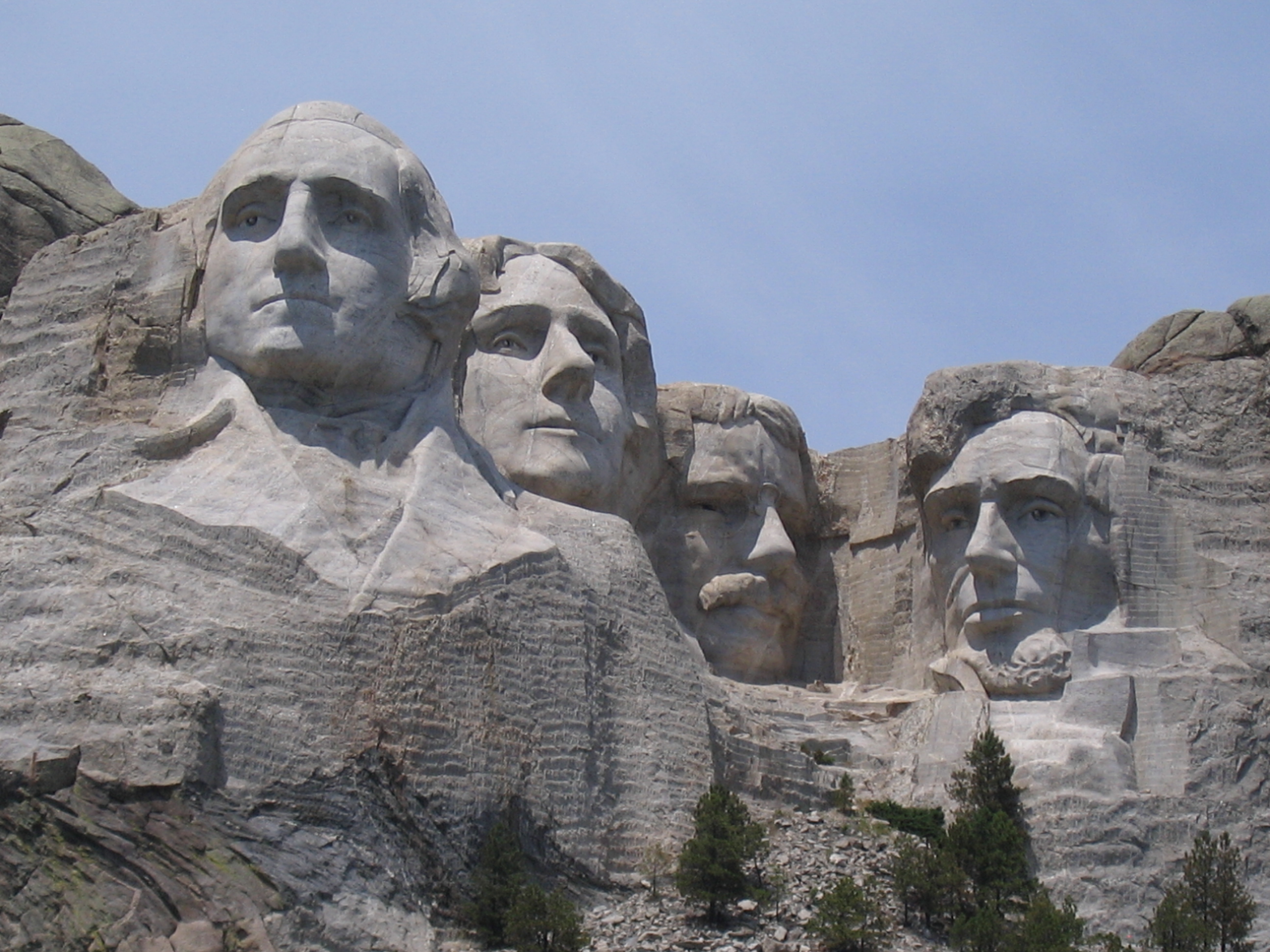
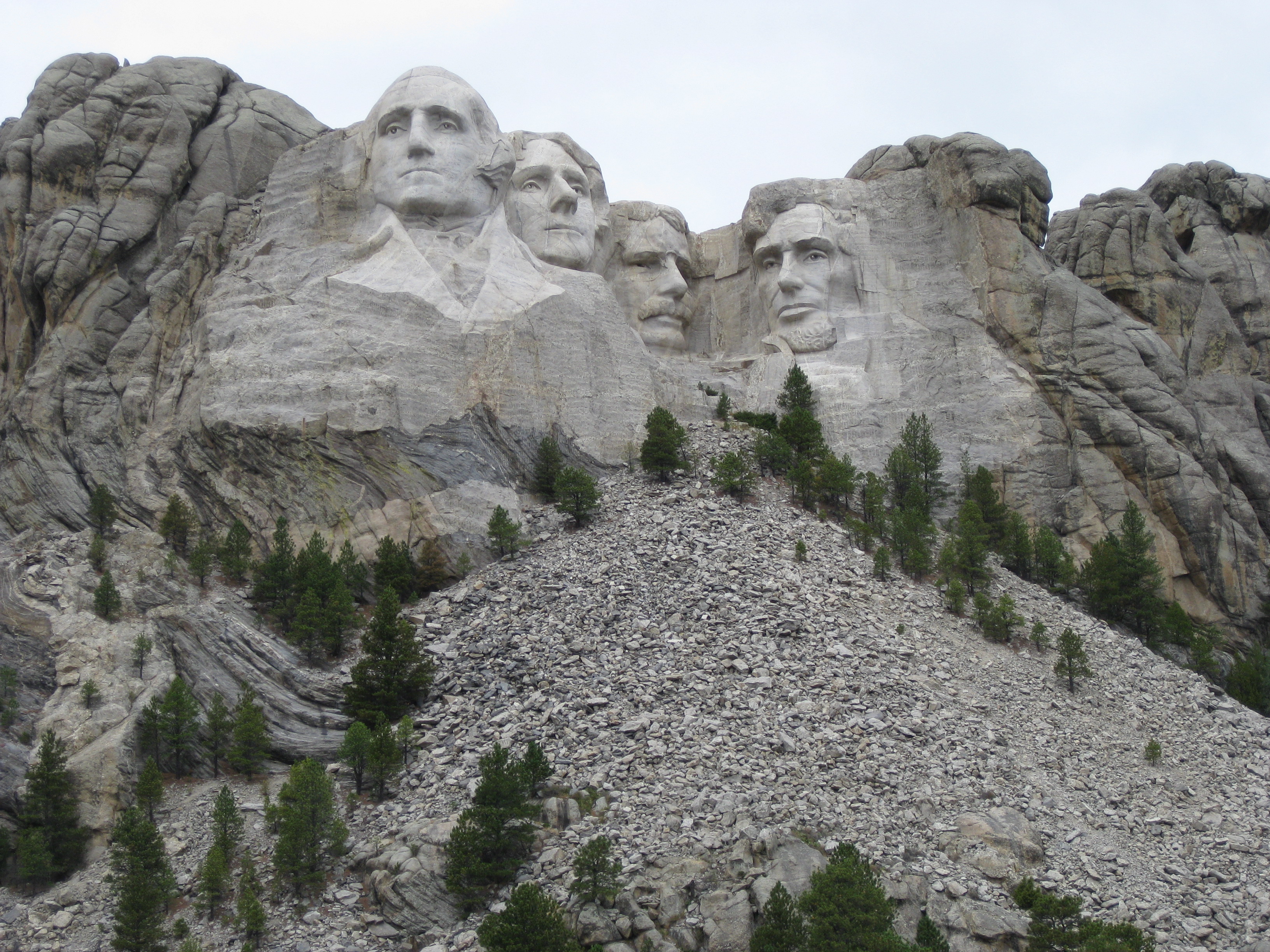
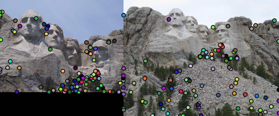
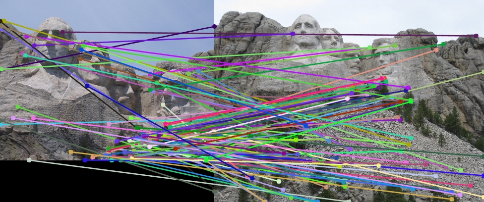
I have tried experimenting the simple pipeline of SIFT-like features using the harris point detection for cornerness and then constructing SIFT features on various images, just to see as to how they perform. Observe them visually as no ground truth is available.
| Image1 | Image2 | Showing Interest points in images | Showing Correspondence in images |
|
|
|
|

|
|
|
|

|
|
|
|
|
|
|
|
All the work that has been implemented for the project has been presented and discussed above. Feel free to contact me for further queries.
Contact details:
Murali Raghu Babu Balusu
GaTech id: 903241955
Email: b.murali@gatech.edu
Phone: (470)-338-1473
Thank you!