Project 2: Local Feature Matching
For this assignment I implemented local feature matching using the sift pipeline. The system is to be able to locate descriptive features in two images with different views of the same scene. The system then matches the descriptors between the two images. My implementation of this system was broken up into four parts:
- Implementation of the Harris corner detector
- Implementation of extraction of SIFT like local features at interest points
- Implementation of the matching algorithm
- Extra Credit: Lowered the dimensionality of the feature vectors using PCA
Harris Corner Detector
First I created the derivate filters for the x and y directions. Then I convolved these filters with the image to get the gradient in the x and y directions. Then I smoothed these image derivatives using a Gaussian filter. I then calculated the Harris corner image using these images and an alpha value of .04.
harris = (Ix2.*Iy2 - Ixy.^2) - 0.04*(Ix2 + Iy2).^2After this I needed to do non-maxima suppression on the harris matrix. I did this by suppressing all values under a threshold of .000005 and taking suppressing all values besides the max value in a sliding window with a size of half the feature width.
SIFT Features
At each interest point I extracted a 16X16 patch and calculated the gradient for that patch. Then for each 4X4 sub-patch I summed the gradients into 8 separate bins based on gradient direction. Then I concatenated the 8 bins of the sub-patches to form a 128 dimensional vector for each interest point.
Matching
For each interest point in the first image I calculated all the matching interest points in the second image. To calculate if two features were a match I looked at the Euclidean distance between the two vectors. Then I looked at the Euclidean distance of the next furthest feature in the second image. I calculated the ratio of distance1:distance2. If this ratio was below above the threshold of .75 then I discarded the match. The confidence value for each match was the inverse of the calculated ratio. Changing the threshold changed the number of matches so if I wanted more matches I simply raised the threshold.
Extra Credit: Creating lower dimensional feature vectors using PCA
The feature vectors for each interest point originally were 128 dimensional. Lowering the dimension of the feature vector allows for faster computation during the distance calculation in the matching process. Using Principle Component Analysis I reduced the vector dimension to 36. To do this I collected 1000, 128 dimensional features from 21 random images of buildings and then computed the principle coefficients. Then I took the top 36 principle components and multiplied them with the feature vectors reducing the size of the vectors to 36.
Results
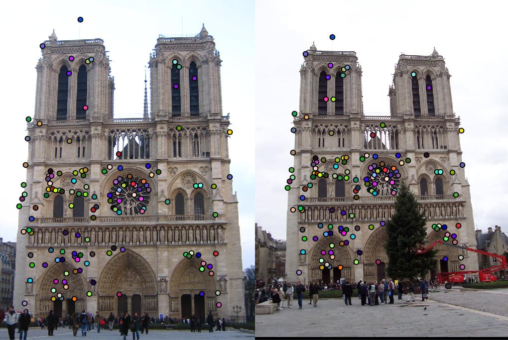
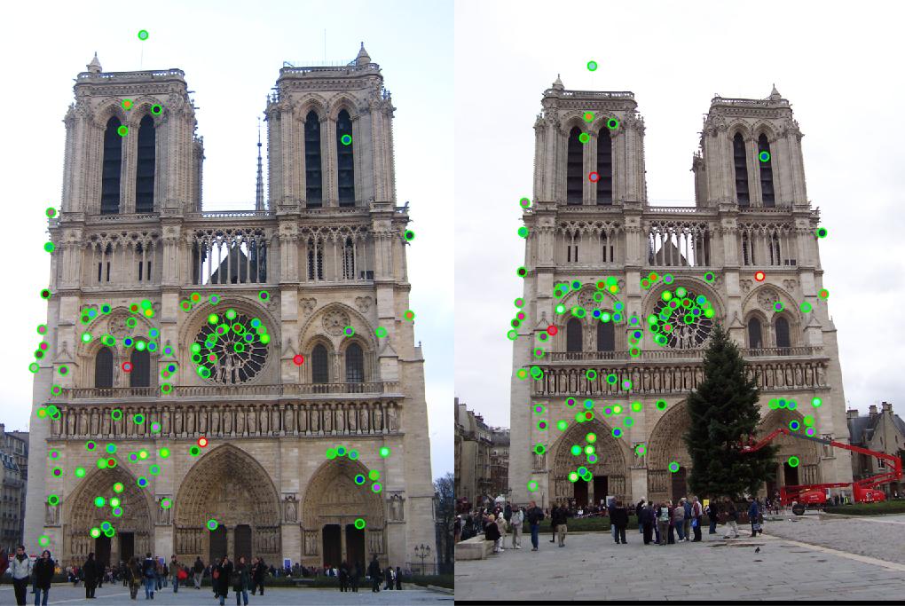
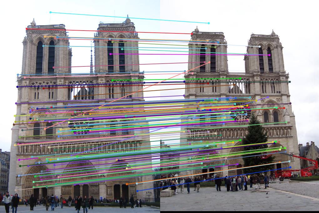
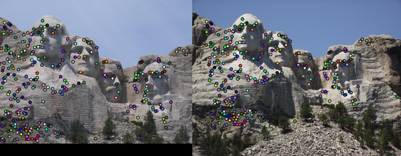
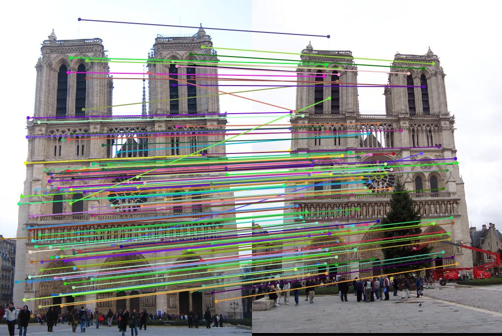
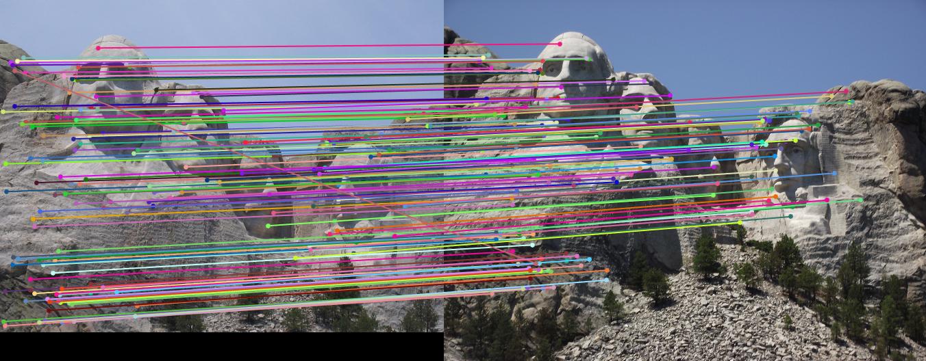
Using the basic homework assignment implementation I got the following results on the three main images for the top 100 matches:
- Notre Dame: 97 total good matches, 3 total bad matches. 0.97% accuracy
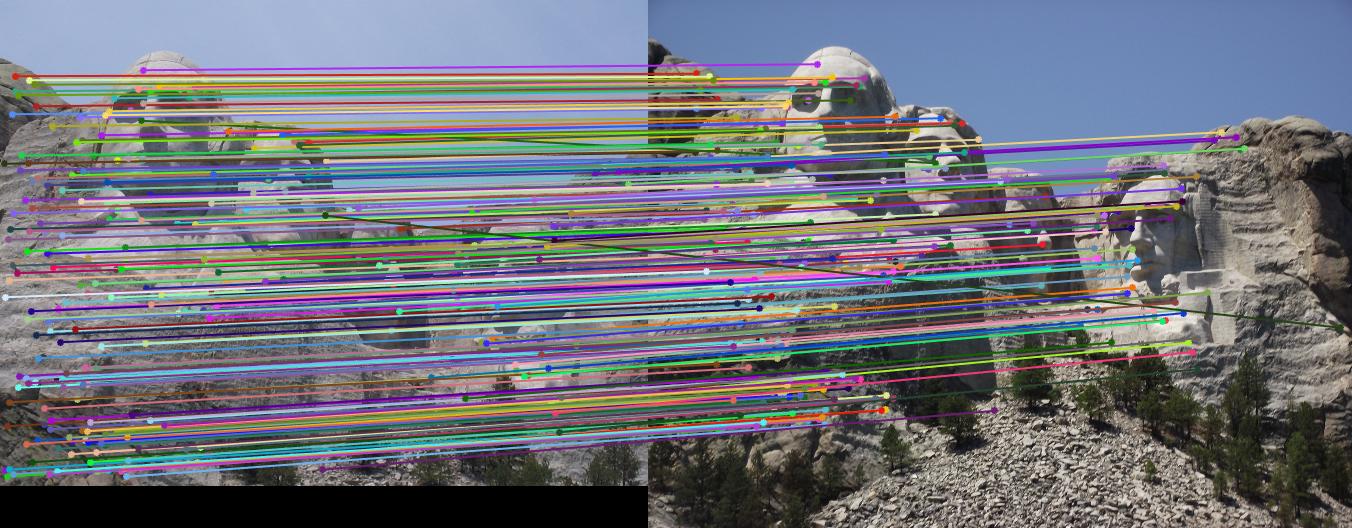
- Mount Rushmore: 100 total good matches, 0 total bad matches. 1.00% accuracy
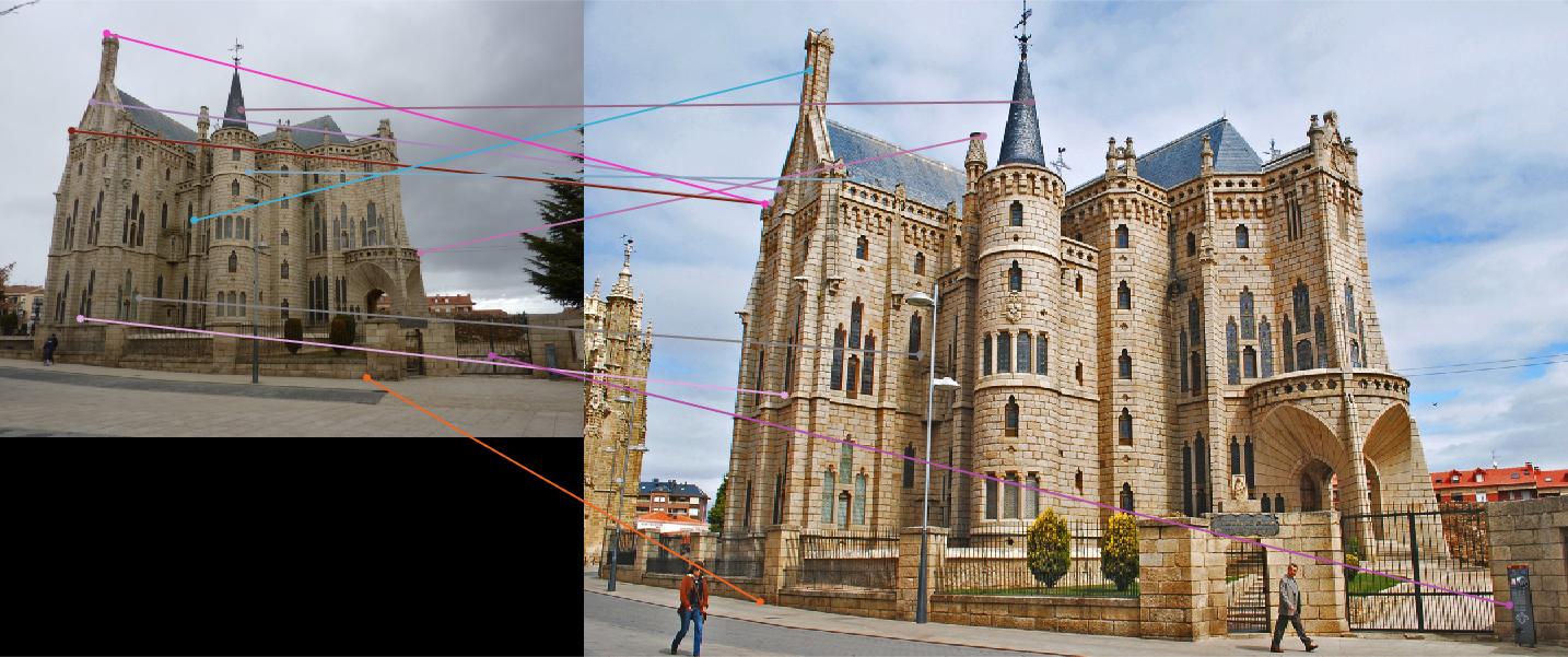
- Episocpal Gaudi: 2 total good matches, 10 total bad matches. 0.17% accuracy (.85 threshold on matches)
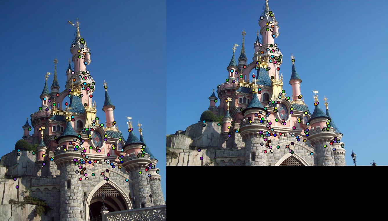
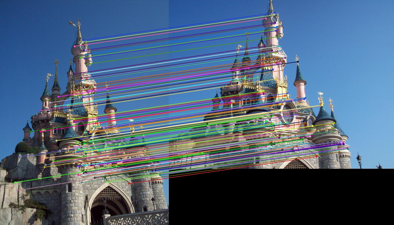
The results of these images run through the pipeline along with an extra photo pair of the Disney park's Sleeping Beauty Castle are shown below.
|
|

|
|
I then implemented the PCA feature dimensionality reduction and ran the pipeline on the Notre Dame and Mount Rushmore images and got the following results:
- Notre Dame: 94 total good matches, 6 total bad matches. 0.94% accuracy
- Mount Rushmore: 99 total good matches, 1 total bad matches. 0.99% accuracy
While there is a slight decrease in accuracy, the results (shown below) look relatively the same and there is a significant reduction of run time of the system.
|