Project 2: Local Feature Matching
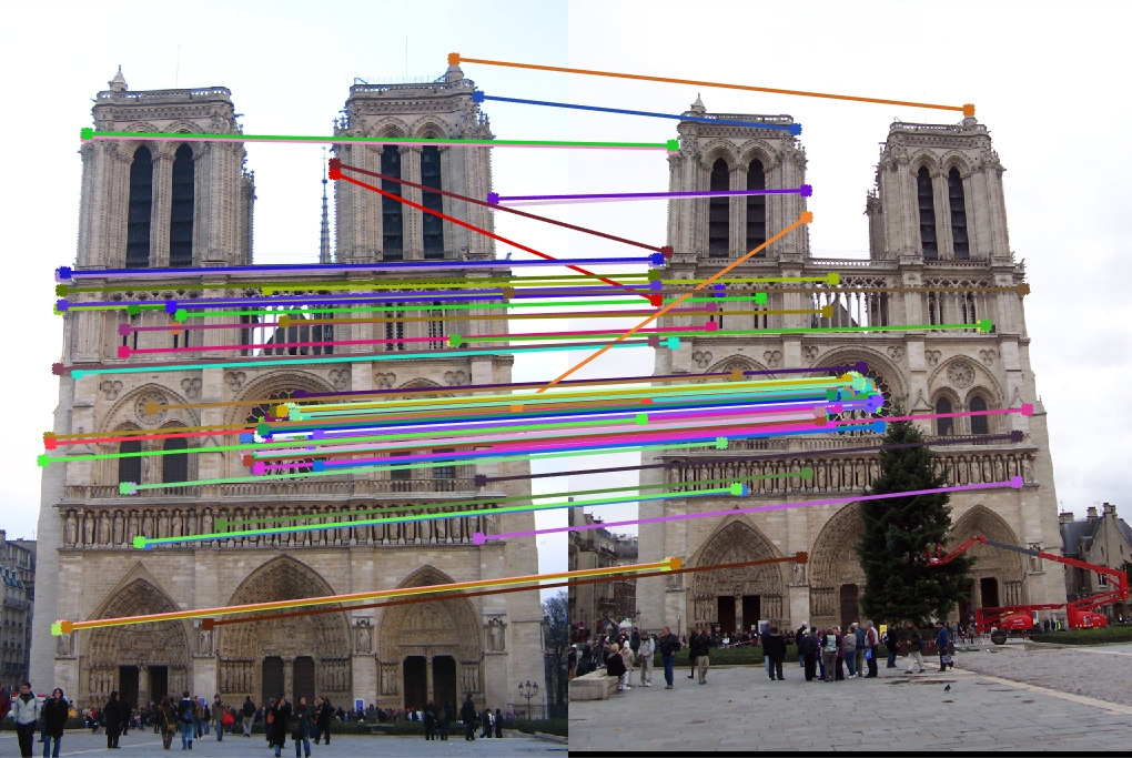
Example of matching points on two Notre Dame pictures.
This project is about creating a local feature mapping algorithm using the knowledge we have so far. The pipeline we base off of is a simplified SIFT pipeline. The project was to implement 3 functions:
- match_features()
- get_features()
- get_interest_points()
I implemented match_features() using the nearest neighbor distance ratio. I found the euclidean distance between features1 and features2 for each feature by using pdist2(), a built in function, to find pair-wise distances. Then I sorted the distances and element-wise divided the smallest by the second smallest distances to get the inverse confidence matrix. Then I set a threshold of .7 (I have tried .6 and .8 but .7 gave me more than 100 good matches with higher than 90% accuracy for Notre Dame pictures while .6 gave me less than 100 good matches and .8 gave me less than 90% accuracy) and set the confidence as element-wise inverse of the inverse confidence if it was less than the threshold. Matches were found by finding where inverse confidence was less than the threshold for x and indices (after sorting) where inverse confidence is less than the threshold. The confidence was found by sorting it in descending order.
I implemented get_features() by implementing a simplified version of the SIFT descriptor. I computed the horizontal and vertical derivatives of the image Ix and Iy by using convolutions. A small gaussian filter then a sobel filter was applied. For Ix, I used the transposed version of the sobel's filter. Then a larger gaussian filter was used to get the gradients. Then I used 3 for loops while iterating through each points to store the histograms in each feature then storing each inside features. I then found the normalized feature with the threshold of .2 for elements. Then I found the inverse of the norm of the feature and multiplied it to the feature to put it into features.
I implemented get_interest_points() with the Harris corner detector. I found the x and y derivative filters using a gaussian filter. The row derivative and column derivative was found using the x and y derivative filters. Using these, I found Ix^2, Iy^2, and Ixy for each layer of the image. Using alpha value of .06 and threshold of .1, I found the Harris corners using the method from the book.
Example Code
match_features()
function [matches, confidences] = match_features(features1, features2)

thresh = 0.7;
distances = pdist2(features1, features2);
[sorted, ind] = sort(distances, 2);

inv = (sorted(:, 1) ./ sorted(:, 2));
confidences = 1 ./ inv(inv < thresh);

ind1 = find(inv < thresh);
ind2 = ind(inv < thresh, 1);

matches = [ind1, ind2];

[confidences, ind] = sort(confidences, 'descend');
matches = matches(ind,:);
end
get_features()
function [features] = get_features(image, x, y, feature_width)

features = zeros(size(x,1), 128);

sigma = 2;
smaller = fspecial('gaussian', sigma, sigma);
image = imfilter(image, smaller);
larger = fspecial('gaussian', 2 * sigma, 2 * sigma);
sobel = fspecial('sobel');

Ixg = imfilter(imfilter(image, sobel'), larger);
Iyg = imfilter(imfilter(image, sobel), larger);
invtan = ceil(4 * (atan2(Iyg, Ixg) / pi + 1));
Ixyg = sqrt(Iyg .^ 2 + Ixg .^ 2);

for n = 1:size(x)
    xn = x(n);
    yn = y(n);
    feature = zeros(1, 128);
    subInv = invtan(yn - 8 :yn + 7, xn - 8:xn + 7);
    subIxyg = Ixyg(yn - 8:yn + 7, xn - 8:xn + 7);

    for i = 0:3
        for j = 0:3
            invtanPatch = subInv(4 * i + 1:4 * i + 4, 4 * j + 1:4 * j + 4);
            IPatch = subIxyg(4 * i + 1:4 * i + 4, 4 * j + 1:4 * j + 4);
            start = 8 * (4 * i + j);
            for k = 1:8
                pix = sum(IPatch(invtanPatch == k));
                feature(1, start + k) = pix;
            end
        end
    end

    normF = 1 / norm(feature, 1);
    feature = feature * normF;
    thresh = 0.2;
    feature(feature > thresh) = thresh;
    normF = 1/norm(feature,1);
    feature = feature * normF;
    features(n,:) = feature;
end
end
get_interest_points()
function [x, y, confidence, scale, orientation] = get_interest_points(image, feature_width)

x = [];
y = [];
[r, c, lay] = size(image);
sigma = 2;
filter = fspecial('gaussian', 2 * sigma + 1, sigma + 1);

xDerivFilt = imfilter(filter, [1,-1], 'symmetric');
yDerivFilt = imfilter(filter, [1;-1], 'symmetric');
rDeriv = zeros(r,c,lay);
cDeriv = zeros(r,c,lay);
Ix2 = zeros(r,c,lay);
Iy2 = zeros(r,c,lay);
IxIy = zeros(r,c,lay);

f = fspecial('gaussian', sigma + 1, sigma);
for l = 1:lay
    rDeriv(:,:,l) = imfilter(image(:,:,l), xDerivFilt);
    cDeriv(:,:,l) = imfilter(image(:,:,l), yDerivFilt);

    Ix2(:,:,l) = imfilter(rDeriv(:,:,l) .^ 2, f);
    Iy2(:,:,l) = imfilter(cDeriv(:,:,l) .^ 2, f);
    IxIy(:,:,l) = imfilter(rDeriv(:,:,l) .* cDeriv(:,:,l), f);
end

a = 0.06;
thresh = 0.01;

harris = Ix2 .* Iy2 - IxIy .^2 - a * (Ix2 + Iy2) .^2;
harris(1:feature_width,:,:) = 0;
harris(end-feature_width:end,:,:) = 0;
harris(:,1:feature_width,:) = 0;
harris(:,end-feature_width:end,:) = 0;
maximum = max(max(harris));
corner = harris .* (harris > thresh * maximum);
res = colfilt(corner, [3 3], 'sliding', @max);
corner = corner .* (corner == res);
[yl, xl] = find(corner);

x = [x; xl];
y = [y; yl];
end
Results in a table
|
|


|
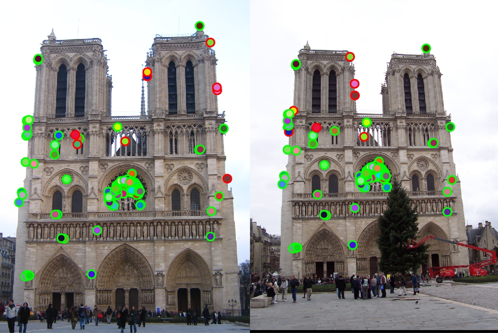
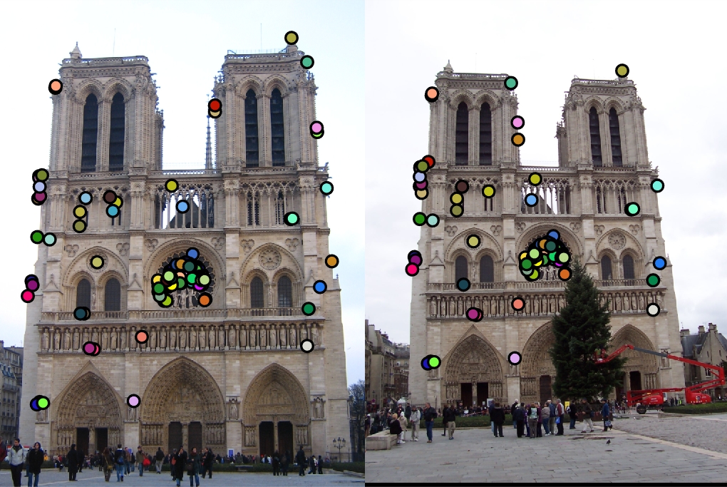
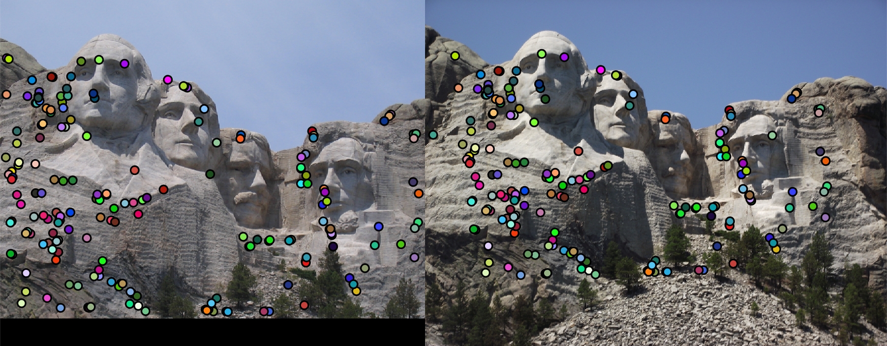
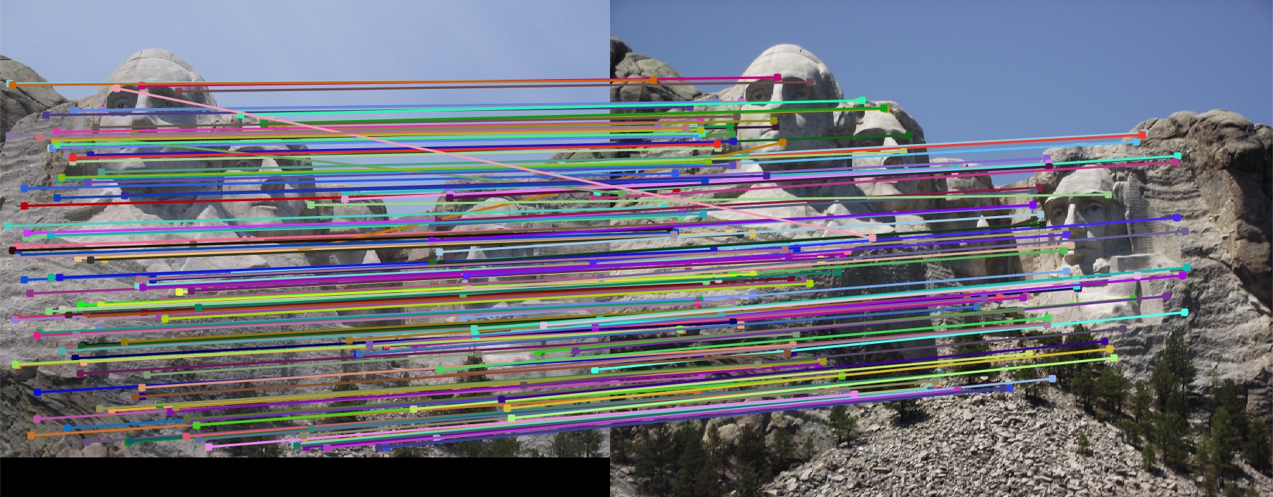
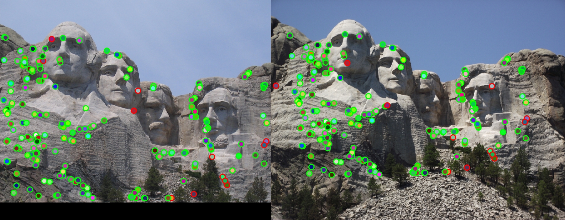
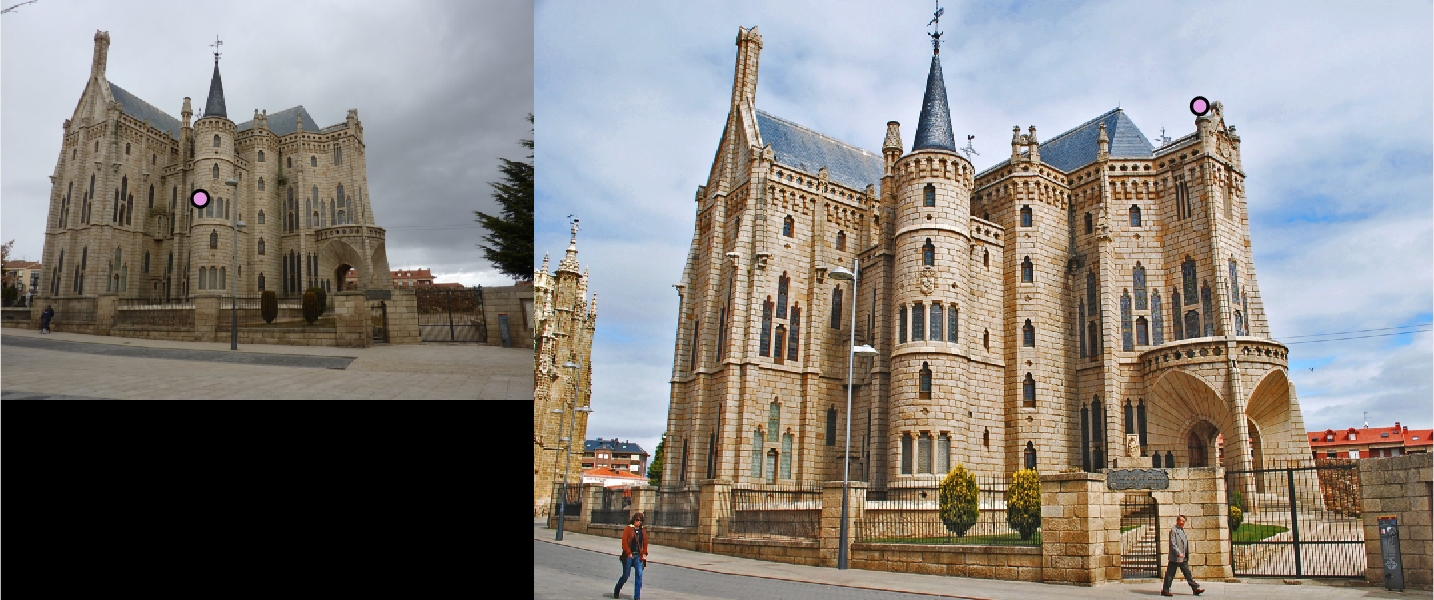
The the pictures in the table are the results of running my version of the simplified SIFT pipeline. The image in the first column is what the algorithm found as distinct interest points. The image in the second column is what the algorithm found as feature vectors at each interest point. The image in the last column is what the algorithm found as matching features. The first row is the result of entering two Notre Dame pictures. The accuracy score came out to be about 93% with 113 good matches and 9 bad matches. The second row is the result of entering two Mount Rushmore pictures. The accuracy score came out to be about 94% with 181 good matches and 12 bad matches. The last row is the result of entering two Episcopal Gaudi pictures. The accuracy score came out to be 0% with 0 good match and 1 bad match.
After playing around with the threshold and sigma values, I tried to maximize my accuracy while finding the most good points as possible (meaning over 100).
The reason the third row, Episcopal Gaudi, was a failure according to this algorithm is because it is hard to find distinct interest points. The building has many similar structures so the algorithm has a hard time finding points. This is unlike the first row, Notre Dame, because the Notre Dame picture had the center where it was clearly distinct. Mount Rushmore also has clearly distinct points so the algorithm was able to find points.