Project 2: Local Feature Matching
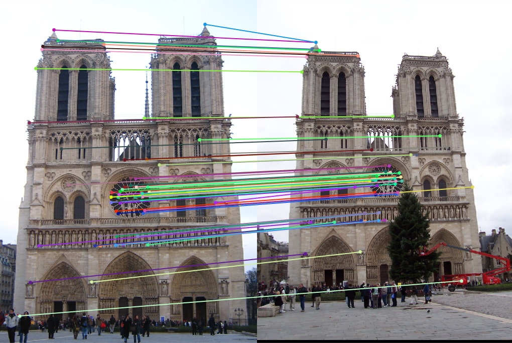
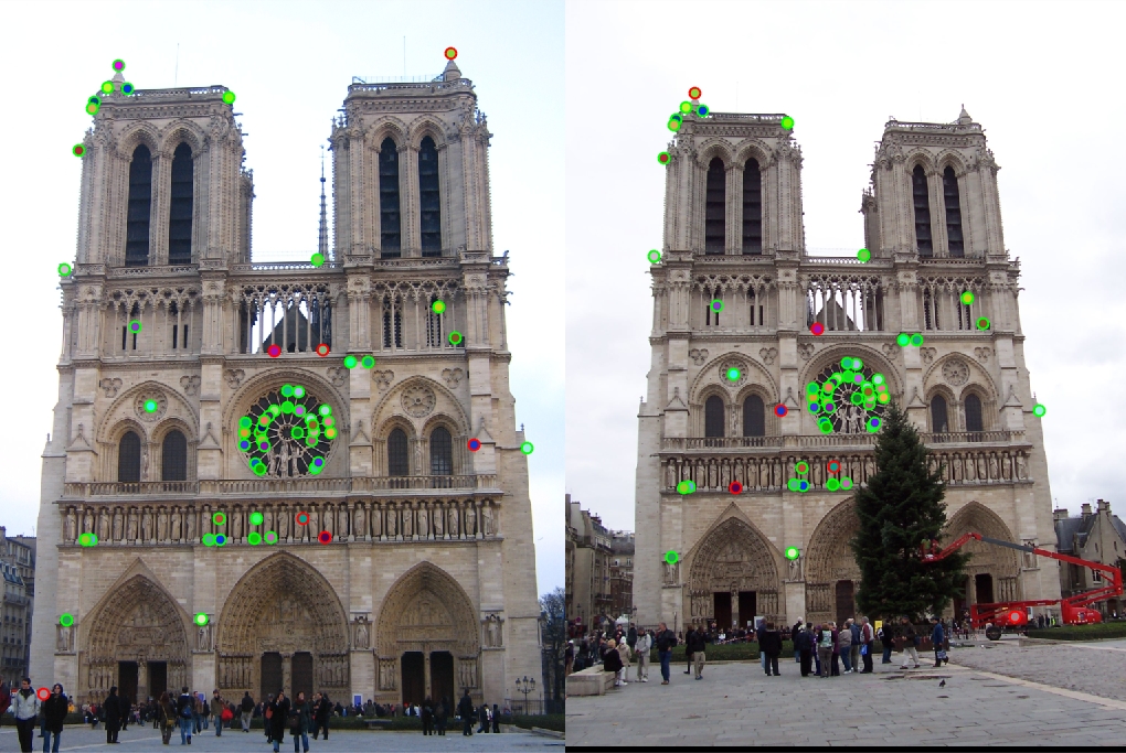
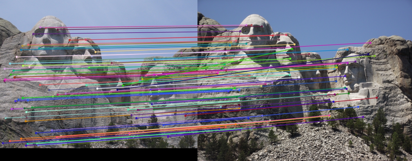
In this example, we had an 88 percent accuracy rating with 52 good matches and 7 bad matches.
This project required me to create a local feature-matching algorithm for similar images. The code took in 2 pictures of the same location and feature matched it based on similar points. After choosing similar interest points, a feature descriptor for all the interest points was created. finally, we found the similarities between the interest points and mapped them. This entire process is similar to the SIFT pipeline but a more simplified version of it.
Algorithm
Part One: Getting Interest points
this part requires the implementation of the harris corner detection implementation. The textbook algorithm requires a few parts that was implemented in my final code.
- Compute the horizontal and vertical derivatives of the image. Do this by doing the derivatives of Gaussians. We could see this in our currentX and currentY values in our code.
- Evaluate the images corresponding to the outer products of their gradients.
- Now we need to convolve the images with a large Guassian.
- Get a scalar interest measure.
- Get the local maximum above the certain threshold that works best.
From my code below, we could see these steps are integrated in the code. Once we got the derivatives of the image and evaluated, we needed to process the gradients that were the near edges using as shown in the edge variable when appropriate zero's were added. The last step was also extremely important where we needed to get the local maximum above the threshold. Using a colfilt with a sliding block type was crucial. The sliding helped with rearranging the m by n sliding neighborhood of the image into a column in a temporary matrix. After that occurred, the function fun would run. This helped take out a lot of the complexity.
//getting the information of the images and computing the derivatives here.. See code for full implementation.

//this edge filtering helps with the processing of the gradients near the edges and sets to zero were neede.
edge = xFiltered .* yFiltered - xyFiltered .* xyFiltered ...
    - 0.04 * ((xFiltered + yFiltered) .* (xFiltered + yFiltered));
edge(:, 1:feature_width) = 0;
edge(:, end-feature_width:end) = 0;
edge(1:feature_width, :) = 0;
edge(end-feature_width:end, :) = 0;

//the below was crucial as explained above.
edge = edge .* (edge > 0.02 * max(max(edge)));
edge = edge .* (edge == ...
    colfilt(edge, [3 3], 'sliding', inline('max(x)')));
Part Two: Getting the features
this part requires the implementation of a feature descriptor for the set of interest points given. We begin by calculating the magnitude and direction of the arrow in each "box" of the array. After that occurs, we need to run through the 4 by 4 array for each value in x. Since we have 8 orientation and 4 by 4 arrays, we get a total of 128 dimensions. Next, we constructed another 4 by 4 matrix to store the new values. If the current value in the 4 by 4 matrix is the same value as the index, we would store that index in the new 4 by 4 matrix. Below I will highlight the important aspects of the code that was critical in the algorithm for this section. The rest of the algorithm can be seen in the matlab code.
...

mag = sqrt(power(imfilter(image, Gx),2) + ...
    power(imfilter(image, Gy),2));
dir = mod(round((atan2(imfilter(image, Gy), ...
    imfilter(image, Gx)) + 2 * pi) / (pi / 4)), 8);

...
for current = 1 : length(x):

	...

	for index = 0 : 7
                four = [0 0 0 0;0 0 0 0;0 0 0 0;0 0 0 0];
                for a = 1 : 4
                    for b = 1 : 4
                        currentVal = directionGrid(a,b);
                        if currentVal == index;
                            four(a,b) = index;
                        end
                    end
                end
                features(current, (((xIndex * 32) + (yIndex * 8)) + index) + 1) ...
                    = sum(sum(magnitudeGrid(logical(four))));
    end
end

features(current, :) = features(current, :) / sum(features(current, :));
Part Three: Matching the features
This part requires the implementation of the ratio test to match the local features. For this step, I needed to first calculate the distance between the two points that we are comparing. After calculating the distance, we need to sort these new distances by their rows. We now need to find that threshold that works best for us (which was .60) and check to see if the two distances below that threshold. If it is, we added those rows to our matches and increased our index by another one. The code below will contain the entire algorithm since it wasn't a large implementation.
//initalized variables here

for x = 1 : featureSize

    for y = 1 : distanceSize
        distances(y, :) = power(distances(y, :) - features1(x, :), 2);
    end
    [distList, index] = sort(sum(distances, 2));

    if 0.60 > 1 / (distList(2) / distList(1))
        confidences(currentIndex) = distList(2) / distList(1);
        matches(currentIndex, 1) = x;
        matches(currentIndex, 2) = index(1);
        currentIndex = currentIndex + 1;
    end

    distances = features2;
end
Results in a table
|
|


|
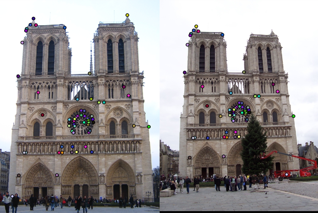
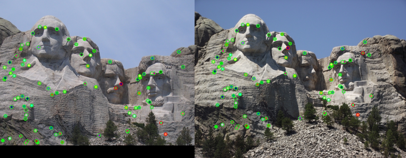
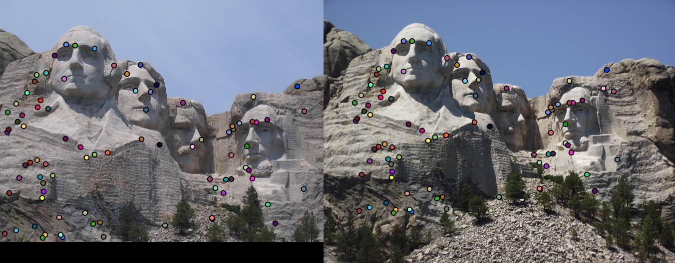
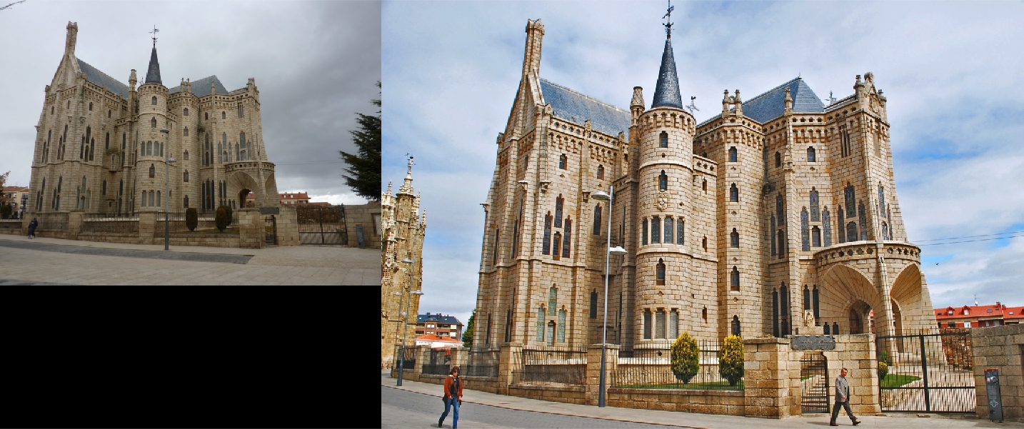
As you can tell from the images above, the Notre Dame image performed well with an 88 percent match success rate. Mount rushmore was, as expected, even higher with a 95% success rate. Unfortunatly, the Episcopal Gaudi did not get any successful matches and I did not want to tackle that issue due to limited time.