Project 2: Local Feature Matching
In this project I have implemented the basic requirements, i.e. a Harris corner detector, SIFT-like features and simple feature matching. Additionally I have done the following bells & whistles:
- Faster matching with kd-trees
- Better spread of interest points with adaptive non-maximal suppression
- MSER as an alternative interest point detection strategy
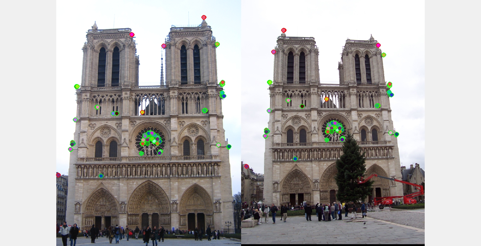
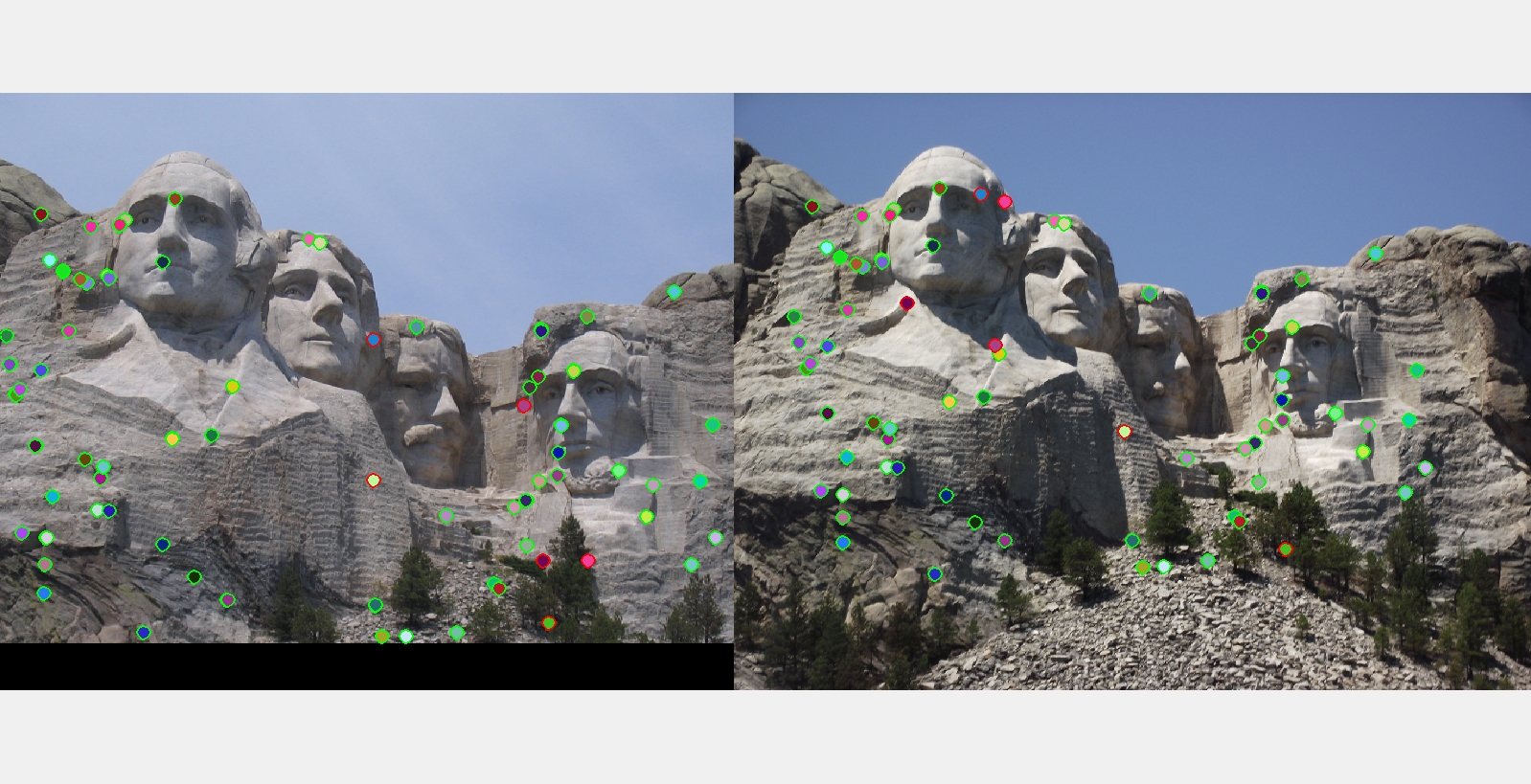
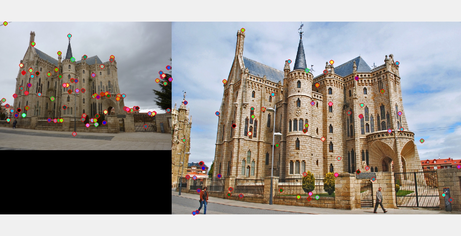
The best matching results I got for each of the three examples with ground truth.
Harris Corner Detector
The implementation is pretty much straight from the slides.
- Gaussian-smooth image
- Compute the derivatives and their products and squares
- Compute the auto-correlation matrix A by smoothing the products and squares
- Compute the cornerness-score for every pixel
- Filter out very weak responses for performance
- Perform non-maximum suppression by comparing each pixel to the interpolated cornerness values along the gradient direction (as explained on the slides)
- Sort the remaining local maxima, i.e. interest points, by their cornerness
Adaptive Non-Maximal Suppression (ANMS)
ANMS continues right where the original Harris corner detector left off. Instead of sorting the interest points by their cornerness value, we sort them by the distance to the nearest neighbor that would suppress them. To understand that we have to take a step back. Normally ANMS takes a radius r as a parameter and suppresses all local maxima that are within a distance of r from another local maximum that is even greater. In the ANMS paper the authors suggest that one should "robustify" this by not only requiring greater but at least 10% greater, which is what we do.
We have modified this as described in the text book. Instead of truly suppressing interest points, we keep all of them but ordered by the maximum suppression radius at which they would first appear. The implementation is exactly that without any optimizations. Szeliski hinted at one where you would first sort the points by their response strength. However, I could not figure it out from just one sentence alone and settled for a runtime of O(n²).
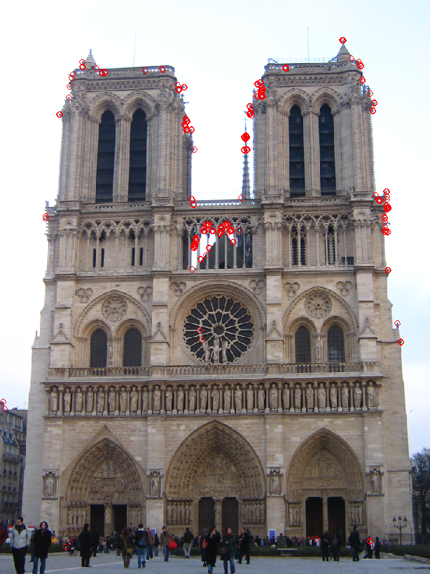
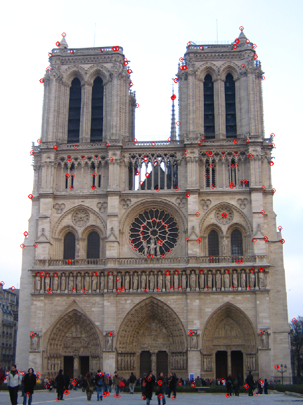
On the left we see the top 250 interest points as found by the default harris detector and on the right are top 250 interest points but selected by the harris detector with ANMS. Obviously the interest points in the right image are very evenly spaced out. This gives the program more chances to find a match in contrast to the situation on the left where interest points are clustered and most likely the program matches either all or none of them.
Maximally Stable Extremal Regions (MSER)
MSER tries to select regions as interest points that have a strong contrast to their surroundings because these ought to be easily found again in other perspectives of the same scene. The algorithm is as follows (assuming integer intensity levels from 0 to 255).
You start with an empty image. Now you incrementally add pixels from the original image ordered by increasing intensity. That is first you add all black pixels, then all pixels with intensity 1/255 and so on. Throughout this process you maintain a list of connected components and their sizes. When you are done, you have a history of connected components as they developed and merged and how their size changed.
From this history you can find the high-contrast regions by looking for connected components that do change in size very slowly over several iterations, since that means that there is a significant jump in intensity between the region and its surroundings. However, this only really works if you also use the MSER features which we did not.
Instead we ordered the regions by two different methods. The first orders the regions by the length of the "reign" of their root pixel. We define reign as the number of iterations between the foundation of a component by its root pixel and its end when it merges with a larger region. The graphs in the last section call this mser-reign. Secondly we also tried to order regions by the longest run of iterations in which they received absolutely no change. That is a region that has been unchanged for 8 iterations has a streak of 8. The plots in the last section call this method mser-streak.

This video shows the components (in white) that MSER finds as it progresses through the intensity levels. Each frame adds 5 more intensity levels to the one before. The video starts with no components at all, i.e. completely black, and ends with a white frame that shows that the complete picture has been combined into a single component.
SIFT-like Features
I have just the basic SIFT features with 16x16 windows, 16 4x4 subwindows and 8 direction bins. The code
- computes the gradient magnitude and orientation of each pixel,
- cuts out a 16x16 window around the interest points,
- downweights the gradient magnitudes in each window with a Gaussian,
- smoothly adds the gradients to the closest bins by "reverse" trilinear interpolation
- and finally normalizes the histograms with the extra cap and renormalize step.
Naive Feature Matching
The first version of the feature matching code iterates through all points, computes the pairwise distance to each of them and selects to two closest ones to return and compute the nearest-neighbor distance ratio (NNDR).
kd-Tree Feature Matching
For the matching part I have implemented kd-tree matching with the matlab class KDTreeSearcher. It is equally simple if not simpler than the naive code and performs better in my experiments as well as asymptotically. While the naive code scales as O(n²), the kd-tree code scales as O(n log(n)). At least in theory. From the graph below one could well argue that both implementations belong to the same class.
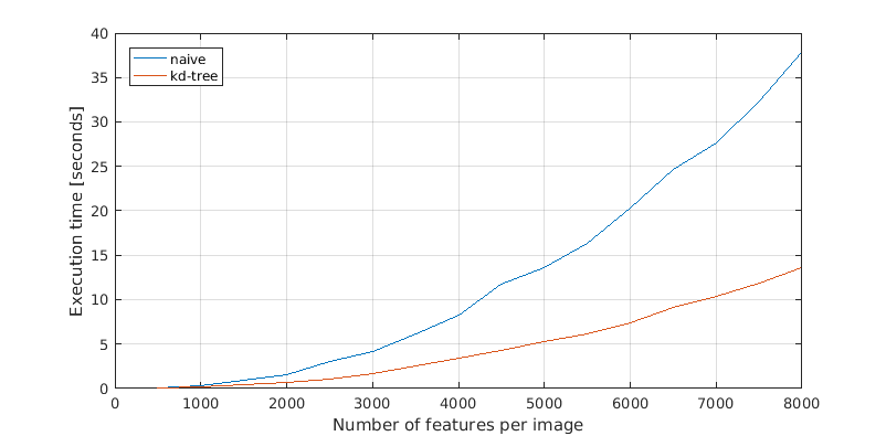
Performance comparison between the naive and kd-tree matching codes on 500 to 8000 features for each image.
Comparing Interest Point Detectors
In this last section we present a comparison between the different interest point detectors. Each plot shows the relation between number of interest points considered and amount of correct matches among the top 100 most confident matches. This means the x-axis shows the number of strongest interest points that we computed features for and considered during matching. Consequently a faster rising line is better as well as one that tops out higher.
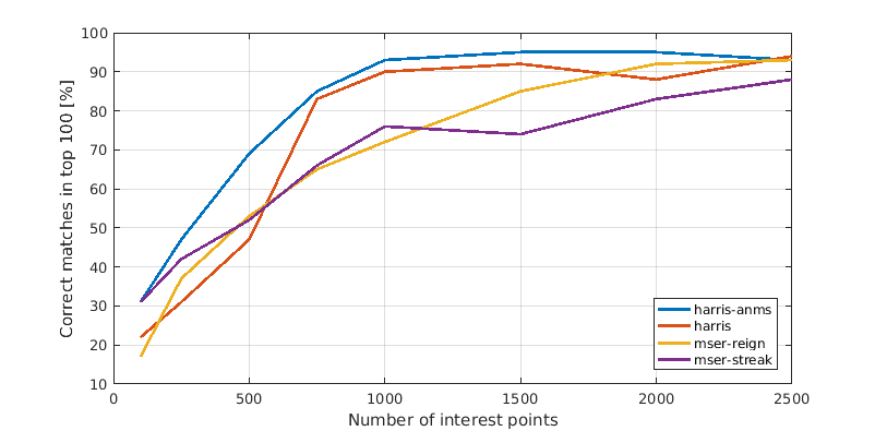
Notre Dame
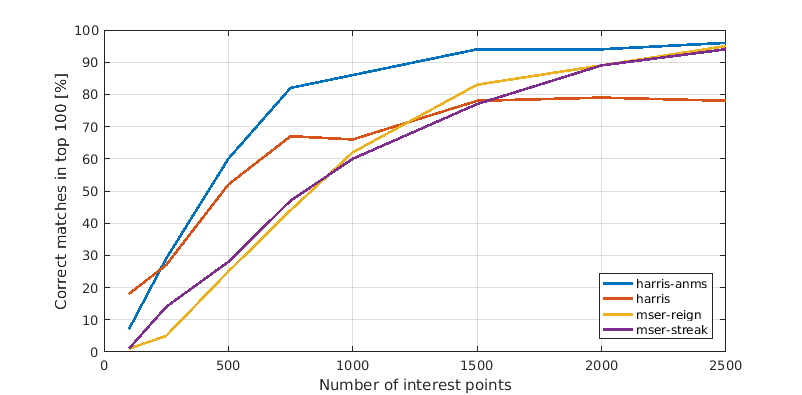
Mount Rushmore
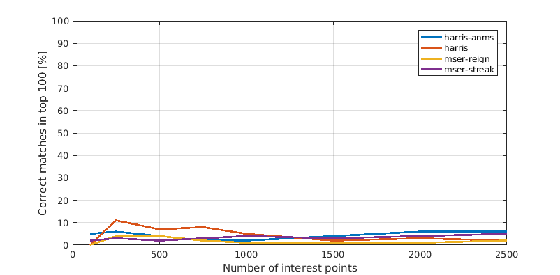
Episcopal Gaudi
In general Harris with ANMS outperformed all others, though it failed just as miserably as everything else on the hardest image. It is surprising that both MSER variations perform relatively weakly. The reason is most likely that you should use the corresponding MSER features, too, for optimal performance.