Computer Vision Project

Project 2: SIFT and Image Matching

Author: Mitchell Manguno (mmanguno3)

Table of Contents
Synopsis
Harris Corner Detection
SIFT
Feature Matching
Results

Synopsis

For this project, an image matching pipeline was implemented, involving interest point detection via Harris corner detection (see here), feature detection via SIFT (see here), and feature matching with a nearest neighbor distance ratio.With this pipeline in place, three pairs of images were matched (two successfully): pictures of Notre Dame, pictures of Mount Rushmore, and pictures of the Episcopal Palace by Gaudí.

I will now explain in detail the corner detection algorithm and its results, the simplified SIFT algorithm used, and the final image results.

Harris Corner Detection

Harris corner detection is a method of detecting interest points in an image by identifying edges and corners in an image. The algorithm is as such:

% optional: blur the image
I = gaussian_blur(image)
% Calculate the derivatives in the x and y direction
I_x, I_y = derivatives(I)
% Square the derivatives
I_x²  = I_x .* I_x
I_y²  = I_y .* I_y
I_xI_y = I_x .* I_y
% Perform a gaussian filter on all squares
g(I_x²)  = gaussian_blur(I_x²)
g(I_y²)  = gaussian_blur(I_y²)
g(I_xI_y) = gaussian_blur(I_xI_y)
% Define some alpha, usually between 0.04 and 0.06
α = 0.06
% Perform the cornerness function
har = g(I_x²)g(I_y²) - [g(I_xI_y)]² - α[g(I_x²) + g(I_y²)]²
% Perform some non-maximum suppression, e.g. max of connected components
components = connected_components(har)
suppressed = zeros(size(har))
for component in components
    maximum = max(component.members)
    suppressed(maximum.coordinates) = 1
end
return suppressed

The above code was implemented in MATLAB, and run to produce the results seen below. You may need to zoom in on the suppressed image to see the selected points.


fig. 1 the original image	fig. 2 after Harris	fig. 3 after suppression

As you can see, the Harris corner detection algorithm detects corners fairly well, and the suppression method pares down clusters of similar points to remove, since they essentially represent the same information.

When implemented, accuracy jumped up about 17% for the Notre Dame pair of images, as compared to the ground-truth comparison points. This is due to the fact that, even though they are not absolutely correct, the sheer number of interest points found resulted in the confidences of the top 100 points to be much higher than the ground-truth equivalents.

SIFT

SIFT is a method of extracting feature information from image data around a point of interest (in this pipeline, the points of interest come from the aforementioned Harris corner detection).

SIFT works by computing the gradient over an image, selecting regions about a feature point, dividing the window up into a 4x4 matrix of 'cells', and placing the magnitude and orientation data for each pixel in the cell into a histogram. These histograms are appended together for all cells in the region to produce feature information for the interest point. The SIFT paper also defines other fine-tuning operations to take place, but, for the purposes of this project, only the base simple features were implemented. The algorithm is as follows:

% calculate the gradient over the image
[magnitudes, directions] = gradient(image)
feature_set = []
% Iterate over all features
for feature in features
    region = feature_width/2 + feature + feature_width/2
    cells = divide(region, [4,4])
    histograms = []
    for cell in cells
        histogram = []
        % Bin the pixels in the histogram based on their direction
        histogram[direction[cell.coordinates]] = magnitudes[cell.coordinates]
        histograms.append(histogram)
    feature_set.append(histograms)
return feature_set

Again, this was implemented in MATLAB. The combined results of this, the Harris corner detector, and the feature matcher will be shown at the end.

After implementation, the accuracy jumped approximately 30% in the Notre Dame pictures (as compared to basic image patches). Ostensibly, this is due to the higher 'density' of information in each feature: magnitude and direction information of pixels is far more informative than simply raw pixel intensities.

Feature Matching

A simple L2 distance-based algorithm was used to find the two nearest matches for each feature in the original image. From this, a confidence score, called the nearest neighbor distance ration, was calculated. It is defined as such.

NNDR = ^d₁ ⁄ _d₂ = ^{D_a - D_b} ⁄ _{D_a - D_c}

Where D_a is the current feature, D_b is its nearest neighbor, and D_c is the second nearest neighbor. The lower this ratio is, the closer we can be sure that D_a and D_b are a match.

Results

As mentioned earlier, this pipeline of Harris-SIFT-NNDR was run on three pairs of images. Two of these pairs were very successful in their matching, while one of them was not. The results are as follows.

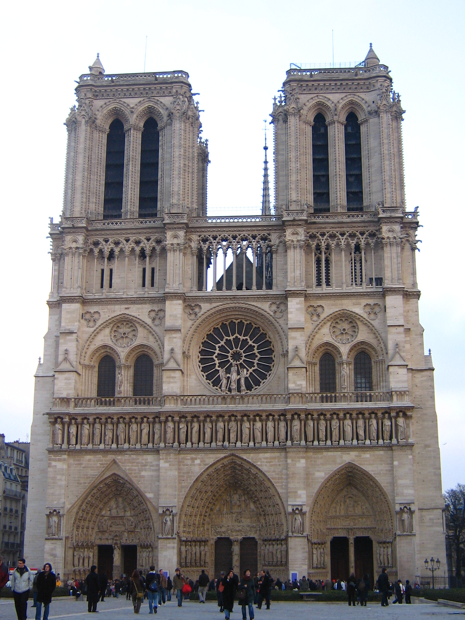
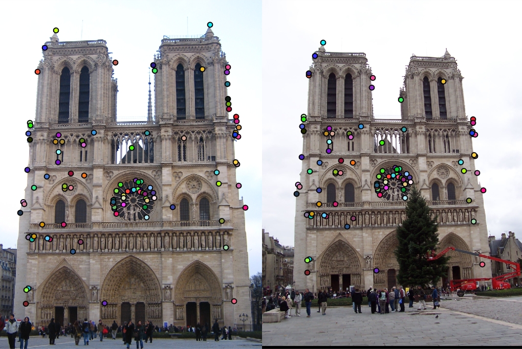
Notre Dame


fig. 4 Notre Dame picture #1	fig. 5 Notre Dame picture #2

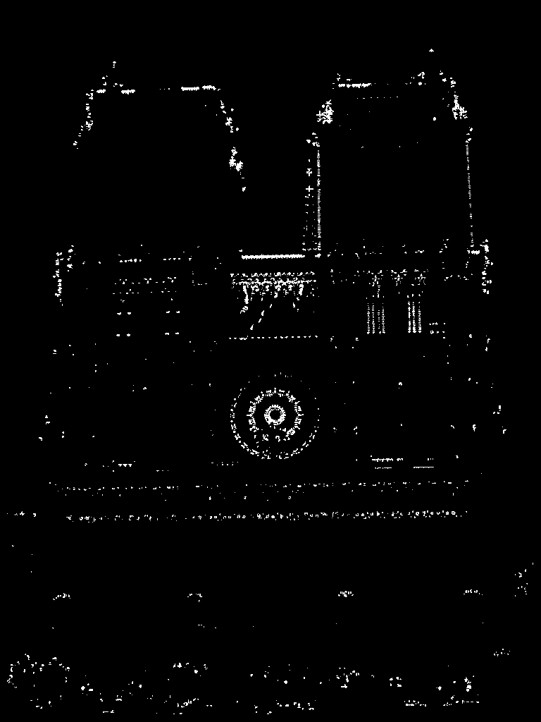
fig. 6 top 100 most confident interest points

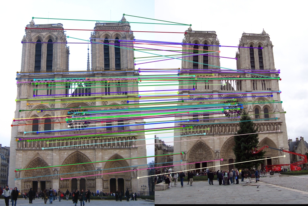fig. 7 matches from points in fig. 4 to fig. 5

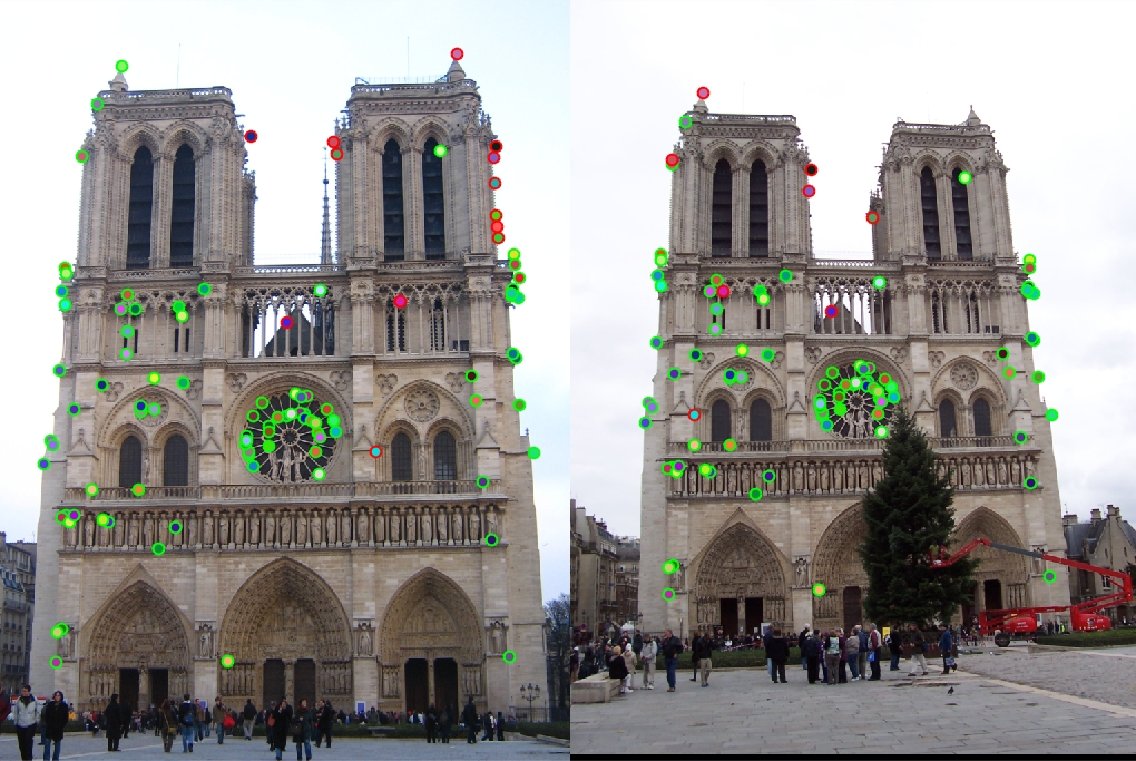fig. 8 evaluated: green outline indicates a successful matching

The Notre Dame pictures matched 87 out of 100 interest points, with a total accuracy of 87%. Much of the successful matching came from the central circular window and the midsection of the building. The entrances, being obscured in the second picture, were not confident enough matches to be considered.

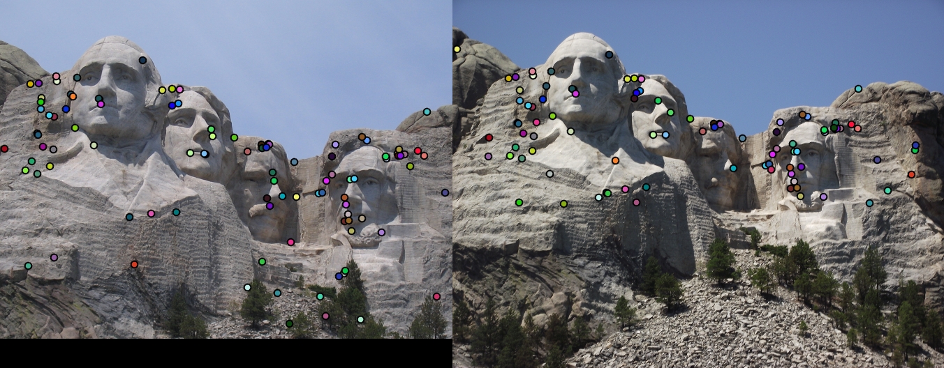
Mt. Rushmore


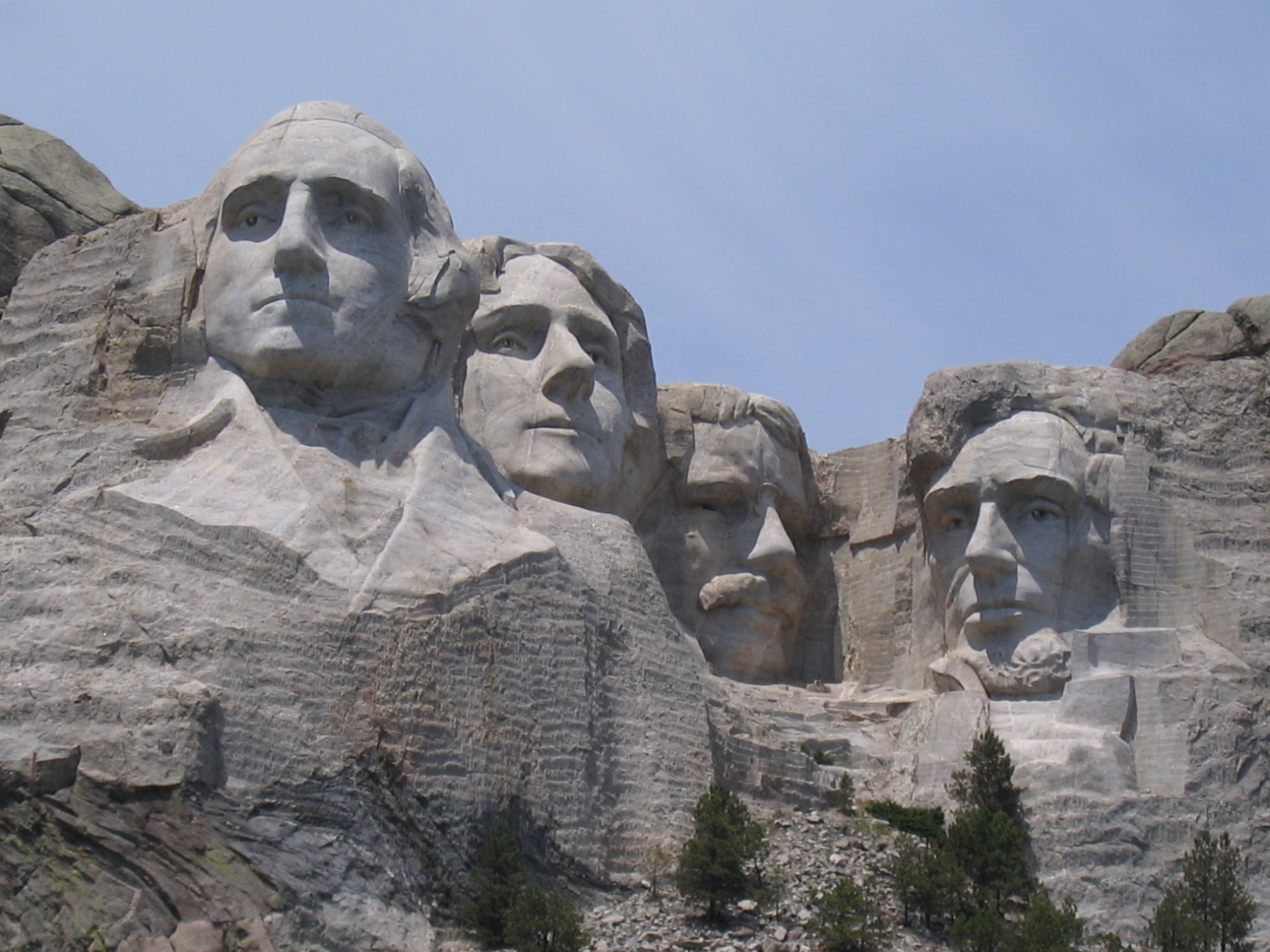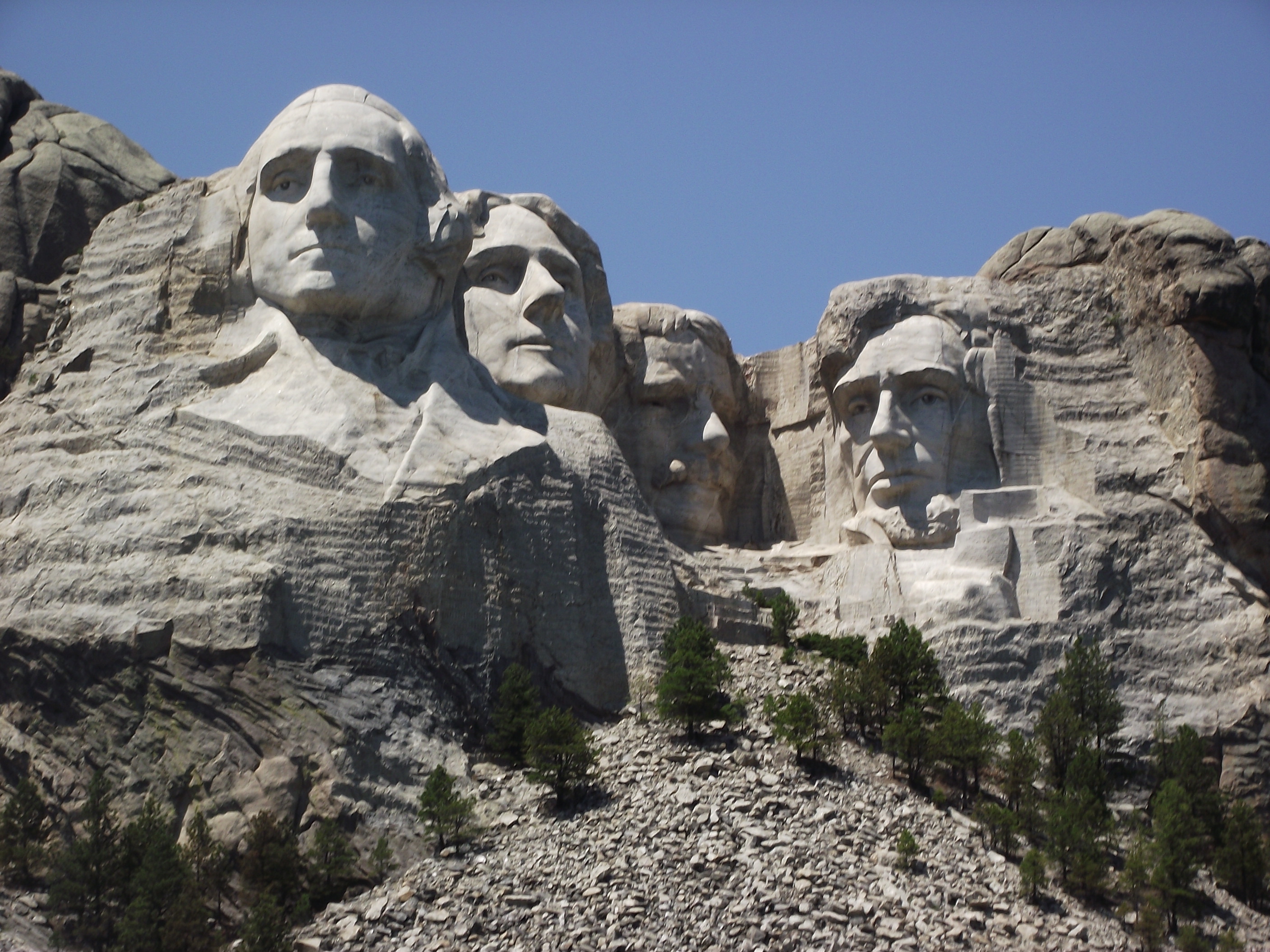fig. 9 Mt. Rushmore picture #1	fig. 10 Mt. Rushmore picture #2

fig. 11 top 100 most confident interest points

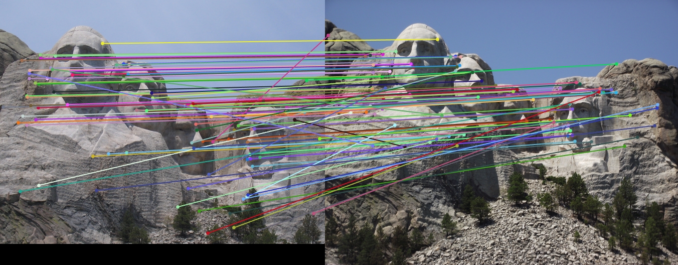fig. 12 matches from points in fig. 9 to fig. 10

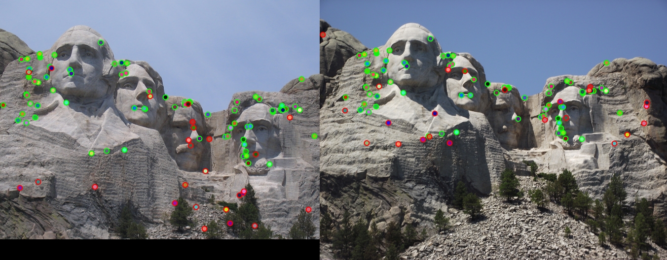fig. 13 evaluated: green outline indicates a successful matching

The Mt. Rushmore pictures matched 74 out of 100 interest points, with a total accuracy of 74%. Most of the successful matches here come from the the left of Washington's face, and Lincoln's face. I assume this is true due to the relative invariance between the features in the two features.

Episcopal Palace by Gaudí


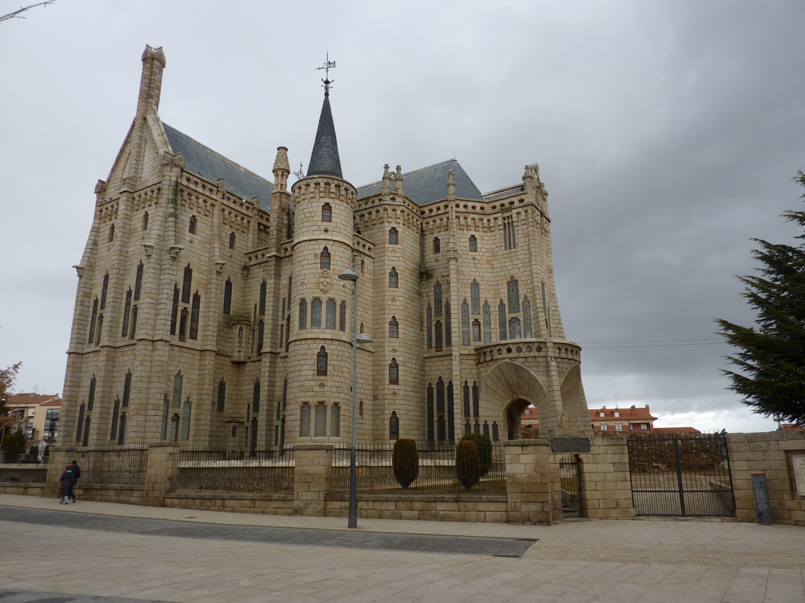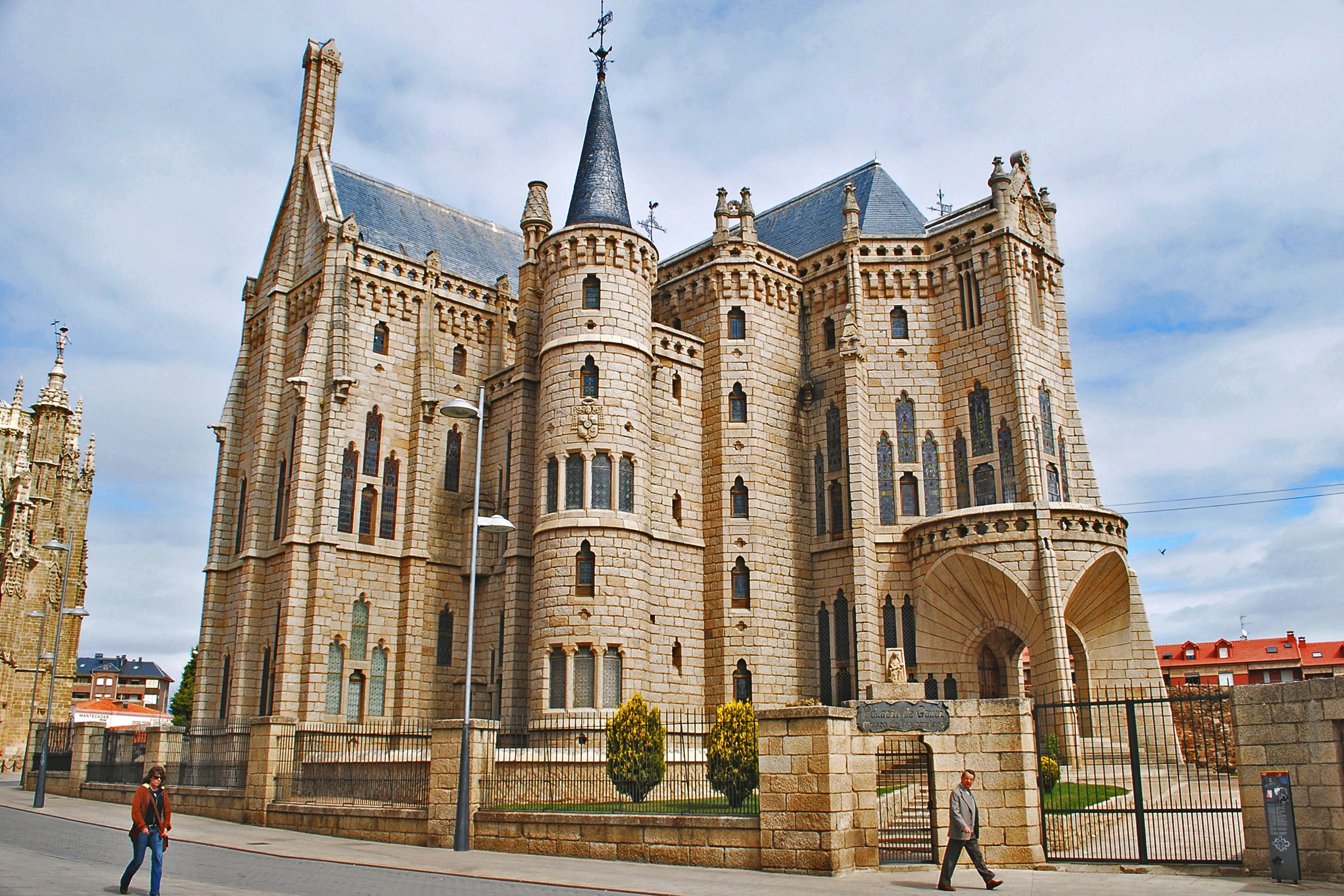fig. 14 Episcopal picture #1	fig. 15 Episcopal picture #2

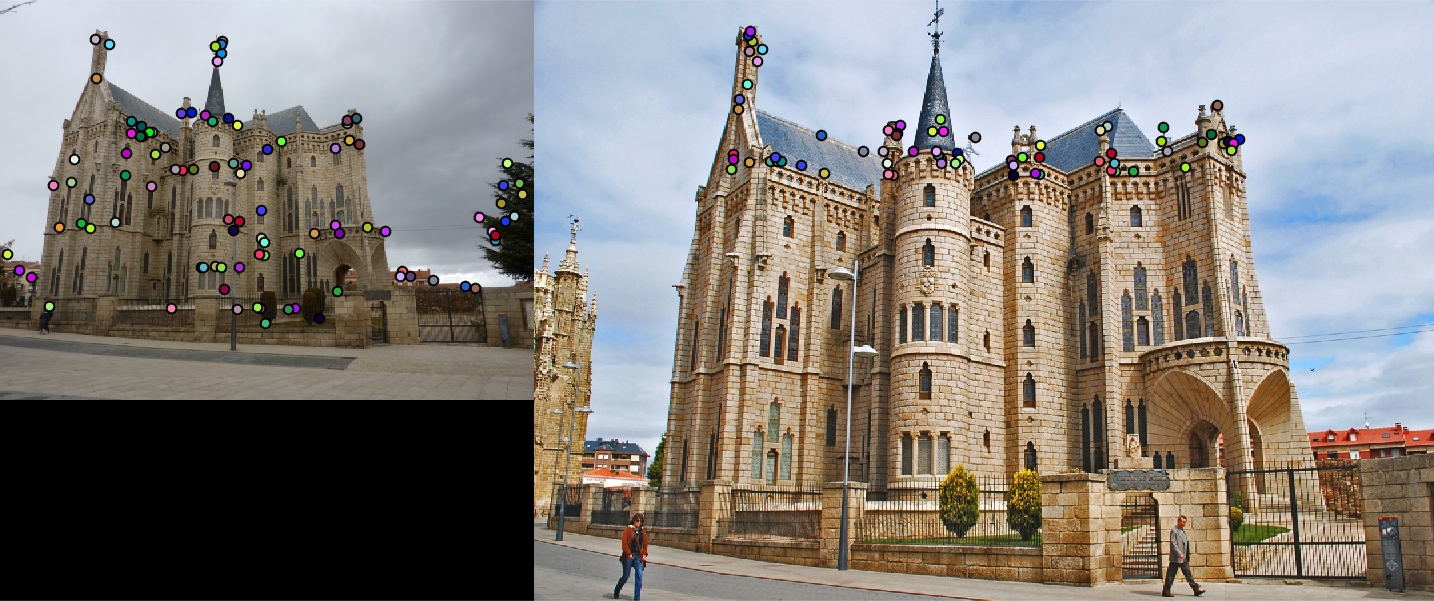fig. 16 top 100 most confident interest points

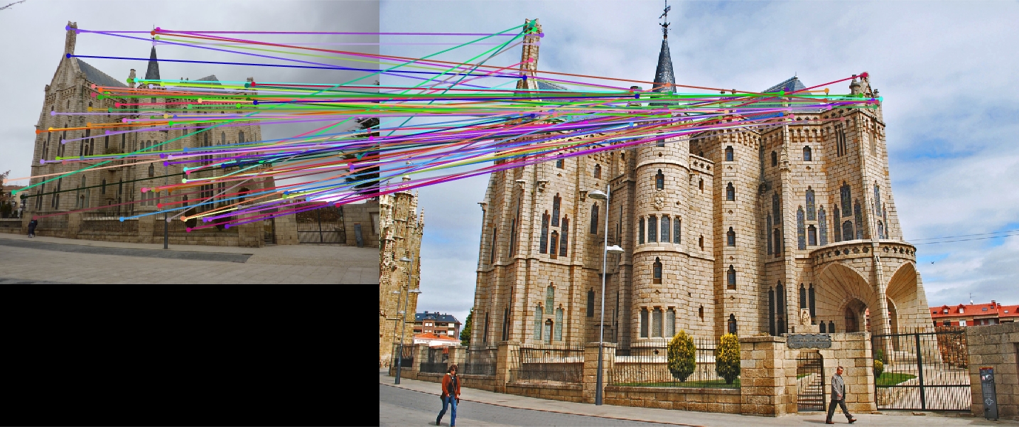fig. 17 matches from points in fig. 9 to fig. 10

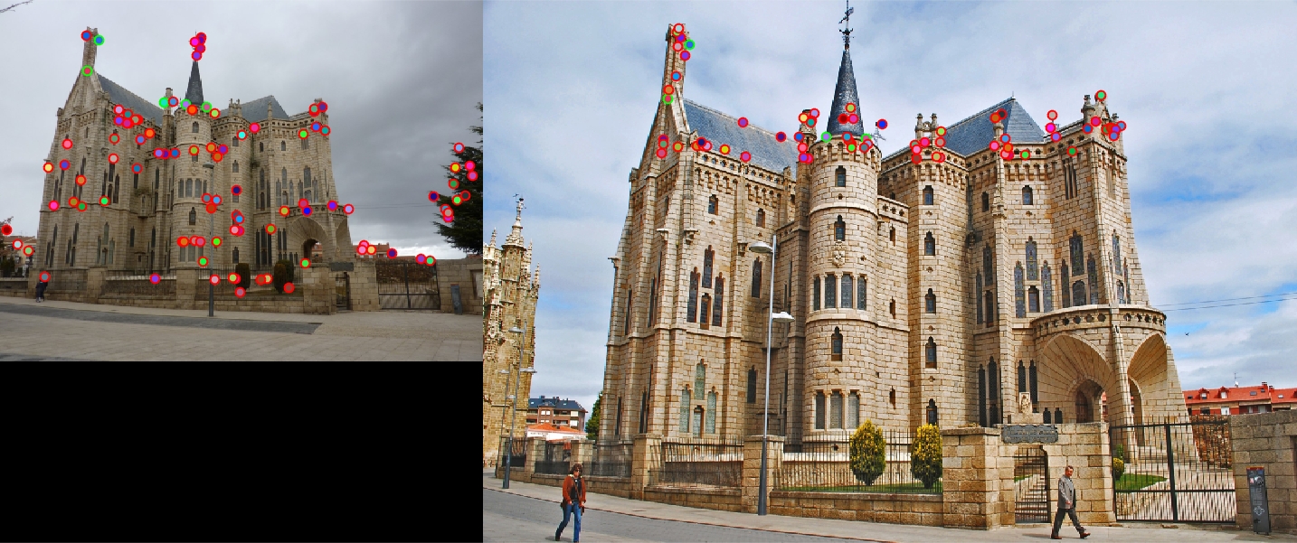fig. 18 evaluated: green outline indicates a successful matching

The Episcopal Palace pictures matched 5 out of 100 interest points, with a total accuracy of 5%. Two major things contributed to the failure of this matching. One, the difference in image size; image #1's size was far smaller than image #2, so the region around the interest points in image #1 was much larger than in image #2 (relative to the total image size). Two, the great difference in color and perspective greatly skewed the feature matching.

Mitchell Manguno