Project 2

Local Feature Matching

In local feature matching, we transform an image into a large collection of feature vectors, each of which is invariant to image translation, scaling, and rotation, partially invariant to illumination changes and robust to local geometric distortion. This is uses to compare any two images containing the same components and successfully match these parts.

The feature matching pipeline comprises of primarily 3 stages :

Interest point detection
Local feature description
Feature Matching

Stage 1: Interest point detection

During the feature detection (extraction) stage, we search each image for locations that are likely to match in other images. Here, we compute the potential keypoints by finding image derivatives in x and y direction, find the squares of derivatives, and apply a gaussian(blur) filter. We compute the Harris corner detector by calculating M matrix for each image window to get their cornerness scores. We then find points whose surrounding window gave large corner response (f> threshold) and take the points of local maxima, i.e., perform non-maximum suppression.



function [x, y, confidence, scale, orientation] = get_interest_points(image, feature_width)

    alpha = 0.05;                                           % define alpha for harris descriptor
    dx = [-1 0 1, -2 0 2, -1 0 1];                          % x-derivative matrix
    dy = dx';                                               % y-derivative matrix
    g = fspecial('gaussian',[1,feature_width], 1);          % define a guassian filter
    [no_of_rows, no_of_columns]=size(image);
    corner_size = feature_width/2 ;

    % compute derivatives
    Ix = imfilter(image, dx , 'same');
    Iy = imfilter(image, dy , 'same');

    % convolve with squares of derivatives and gaussian
    Ix2  = imfilter(Ix.^2, g , 'same');
    Iy2  = imfilter(Iy.^2, g , 'same');
    IxIy = imfilter(Ix.*Iy, g , 'same');

    % Harris cornerness measure
    hcm = Ix2.*Iy2 - IxIy.*IxIy- alpha * [Ix2 + Iy2].^2;

    % Use the colfilt function to find local maxima at each sliding window
    hcm_thresholded=hcm.*(hcm>(graythresh(hcm)/10.0));
    colfilt_result=colfilt(hcm_thresholded,[feature_width feature_width],'sliding',@max);
    hcm_thresholded= (hcm_thresholded==colfilt_result).*(hcm_thresholded);

    % discard indices in the corners
    [r,c]=find(hcm_thresholded);
    for i=1:length(r)
        if (r(i)<=corner_size | r(i)>=no_of_rows-corner_size) | (c(i)<=corner_size | c(i)>=no_of_columns-corner_size)
            hcm_thresholded(r(i),c(i))=0;
        end
    end
    [y,x]=find(hcm_thresholded);
end

Stage 2: Local feature description

We find the SIFT descriptor, which defines the features in an image independent form. Every region around a potential keypoint is converted into a rotation, scale or intensity invariant descriptor. These feature descriptors are stable, reliable and are unique and can be matched against other descriptors. We take 4x4 window of cells, each feature_width/4 where each cell has an histogram of the local distribution of gradients in 8 orientations. Appending these histograms together gives us the feature which is further normalized to unit length. In summary, we take a 16×16 window of “in-between” pixels around the keypoint that is split into sixteen 4×4 windows. From each 4×4 window we generate a histogram of 8 bins. Each bin corresponding to 0-44 degrees, 45-89 degrees, etc. Gradient orientations from the 4×4 are put into these bins. This is done for all 4×4 blocks. Finally, we normalize the 128 values.



% define variable and constants
cell_size=feature_width/4;
half_feature_width = feature_width/2;
histogram_size = 8;
threshold = 0.2;
features=[];

for z=1:length(x)

    % compute the histogram (partial image feature) each time using this variable
    histogram=[];

    r=y(z);
    c=x(z);

    % find the window from the image and convert it from a matric to a cell
    window=image(r-half_feature_width:r+half_feature_width-1, c-half_feature_width:c+half_feature_width-1);
    window=mat2cell(window, ones(1,cell_size)*cell_size,ones(1,cell_size)*cell_size);

    for i=1:cell_size
        for j=1:cell_size

            %Convert back to matrix
            cell=cell2mat(window(i,j));

            % calculate the magnitude and angles
            [mag,ang]=imgradient(cell); 
            
            h=zeros(1,histogram_size);

            % find the image discriptor at each 4*4 window.
            for k=1:cell_size
                for l=1:cell_size

                    % find the angle for each descriptor
                    angle = ang(k,l);
                    if angle < 0
                        angle = 360 + angle;
                    end

                    % find the position in the histogram where this orientation is stored
                    index = floor(angle/45) + 1;
                    h(index) = h(index)+mag(k,l);
                end
            end
            histogram=[histogram h];
        end
    end
    
    % Normalize the hisogram
    d=norm(histogram);
    histogram=histogram./d;

    % Set a cut off threshold
    histogram = min(histogram,threshold);

    % Normalize the hisogram again
    d=norm(histogram);
    histogram=histogram./d;   

    % append to features.
    features=[features;histogram];
end

Stage 3: Feature Matching

In this feature matching stage we search for likely matching candidates in other images. This is done using the nearest neighbor distance ratio (NNDR). In this case, a useful heuristic is to compare the nearest neighbor distance to that of the second nearest neighbor, preferably taken from an image that is known not to match the target, and then only those ratios in a certain threshold are considered as valid matched features.


% MATCH FEATURES USING NNDR
% Psuedocode used to write the algorithm : 
% http://stackoverflow.com/questions/5565225/sift-feature-matching-through-euclidean-distance-matlab-help-pls

size_features_1 = size(features1,1);
size_features_2 = size(features2,1);
euclidian_distances = zeros(size_features_1,size_features_2);

% find the euclidian_distances between each pair of features
for i = 1:size_features_1
    for j = 1:size_features_2
        euclidian_distances(i,j) = norm(features1(i,:)-features2(j,:),2);
    end
end

% sort the distances
[sorted_distances, sorted_indices] = sort(euclidian_distances,2);
nndr_ratio = sorted_distances(:,1)./sorted_distances(:,2)

% cut off at threshold

threshold = 0.7;
thresholded_nndr_indices = find(nndr_ratio (less than) threshold);
matches = zeros(size(thresholded_nndr_indices,1),2);

% get the x and y undices
matches(:,1) = thresholded_nndr_indices;
matches(:,2) = sorted_indices(thresholded_nndr_indices);

% Sort the matches so that the most confident onces are at the top of the
% list. You should probably not delete this, so that the evaluation
% functions can be run on the top matches easily.
confidences = 1-nndr_ratio(thresholded_nndr_indices);
[confidences, ind] = sort(confidences, 'descend');
matches = matches(ind,:);

Extra credit

Implemented SIFT, and used the angles as well to magnitude to define the feature descriptor.
Thresholded the corners for better accuracy.

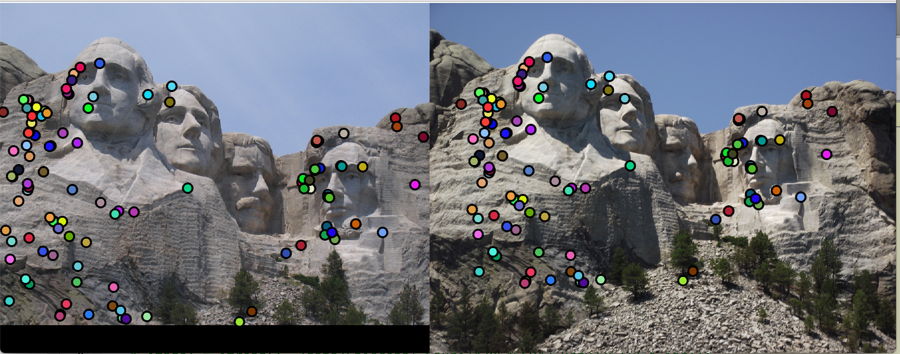
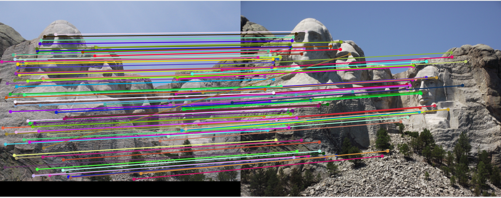
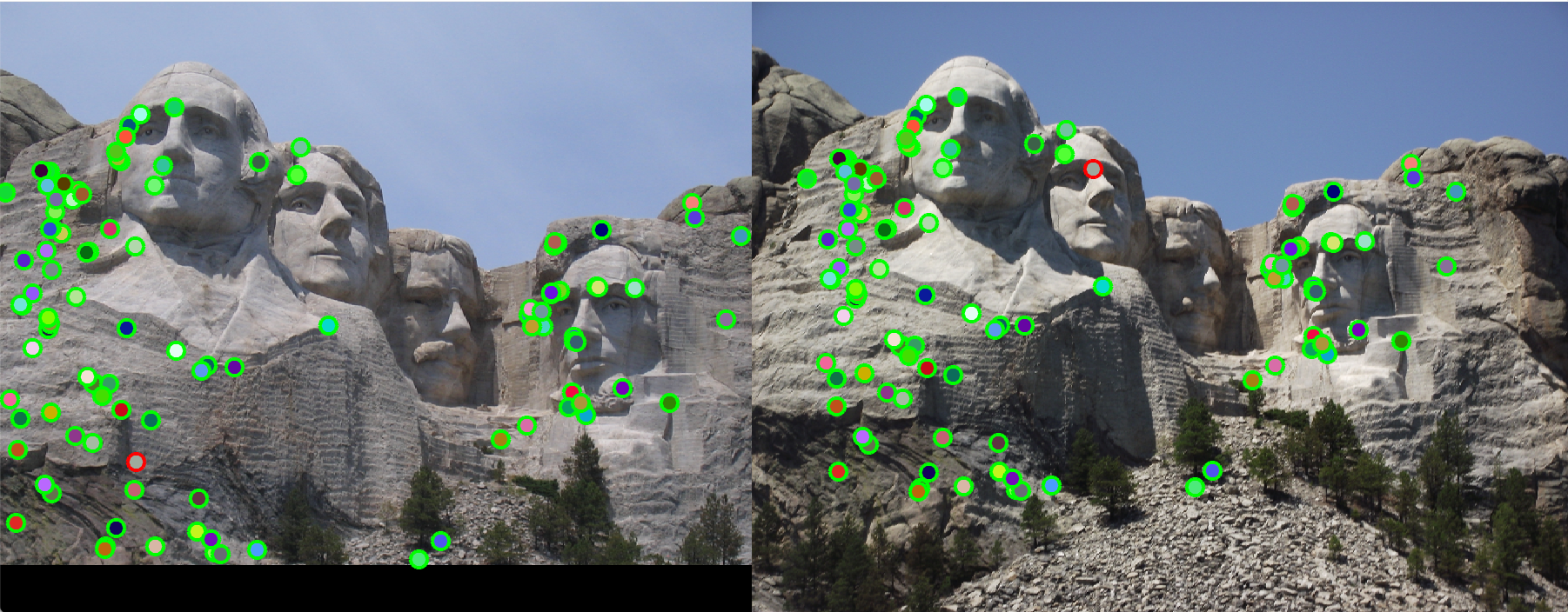
Examples

Below are some examples run over the sample dataset provided.

	Notre Dame	Mount Rushmore
1. Interest point detection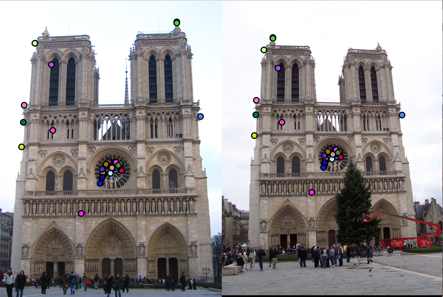
2. Feature Matching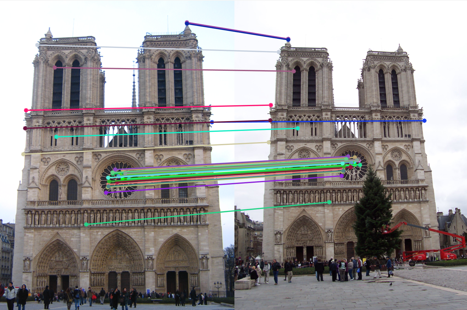
3. Plotting accuracy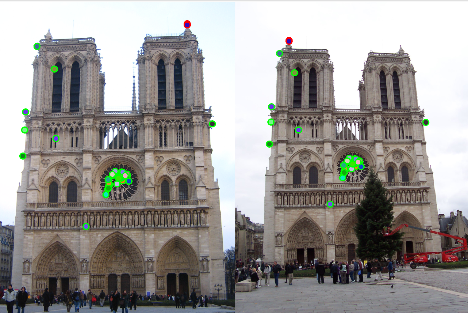