Project 2: Local Feature Matching
This project involves finding similar features between two different images of the same scene. The pipeline used to achieve this, is a simplified version of the SIFT pipeline and it involves the following three stages.
- Get interest points
- Get local feature description at interest points
- Match features
Get interest points
Interest points are those points in an image which are unique and can be easily found out and in the case of this project, even after the image is transformed. Points on edges and flat regions are not easily recognizable when looking through a small window. However points on corners are easily identified, as the intensity changes when moving the window in any direction. Hence corners are useful in finding similar features between two images of the same scene.
In order to find the corners, we use harris corner detection algorithm. This algorithms gives a cornerness score for each pixel in the image. Initially, I blur the image with a 5x5 gaussian filter to remove noise. Then I obtain the horizontal and vertical gradients, Ix and Iy of the blurred image using imgradientxy(). The cornerness function 'har' for the image is computed as:
har = g(Ix^2)*g(Iy^2) - g(Ix*Iy)^2 - alpha*( (g(Ix^2)+g(Iy^2))^2 )
Where alpha = 0.04 and g() is the gaussian filter operation with sigma = 1.5. The chosen values of alpha and sigma were found to give good results. Once we obtain the corners present in the image, we run non-maximum suppression on the corners in order to get only the strongest corners in their respective local neighbourhoods. We use 3x3 window to run non-maximum suppression on the image. Finally after non-maximum suppression, we chose only those strong corners whose cornerness score is >= (mean of the cornerness scores in the image). This is to remove the majority of the corners which are trivial/weak and by this we save valuable computation time in further stages which use corners.
Get local feature description at interest points
We cut out 16x16 patches from the image around the corners obtained from the previous stage. For an initial trial, we normalize these patches and use them as feature descriptors themselves. With this we get around 40% accuracy on the Notre Dame pair. This method suffers from lack of invariance to brightness change, contrast change, or small spatial shifts. We discard this method and move on to implementing a SIFT like feature descriptor for each of the image patches.
Before performing SIFT, we blur the image using gaussian filter to remove noise. We obtained the blurred image's gradient and magnitude using imgradient(). SIFT involves dividing the 16x16 patch of pixels around an interest point into 4x4 cells, with each cell containing 4x4 pixels. Each of these cells have a histogram containing 8 bins, where in each bin is for each 45 degrees of the entire 360 degrees of all the four quadrants. So we have the gradient magnitude and orientation for each pixel in the cell and we split and put the gradient magnitude to the two adjacent bins in which the gradient orientation falls in. The more closer the orientation is to the bin, the higher is the fraction of the magnitude which will be put in that bin. This kind of interpolation is more accurate then sending the entire magnitude to the bin nearest to the orientation. Since each cell generates an eight bin histogram and there are 16 such cells in the entire patch, we finally get a 128 (=4*4*8) element long vector containing all the 8-bin histograms from all the cells of the image patch. Next, the vector is normalized. This is our SIFT like feature descriptor for the image patch which gives much better results than just using normalized image patches.
Match features
In match features, we need to match the two sets of features descriptors of the image pair obtained in previous stage. Here for every feature in one image, we need to find the top two closest matching features in the other image. We use euclidean distance as the metric. Next, we divide the distance between the feature from one image to the closest matching feature from the other image, by the distance between the feature from the first image to the second closest matching feature from the other image. This ratio is denoted as nearest neighbor distance ratio and inverse of this ratio is denoted as confidence measure. We find the confidence measures for the matches for all the feature descriptors of the image pair. The confidences are sorted in descending order and using this sorted list only the top 100 most confident matching features are selected in order to evaluate the accuracy of local feature matching.
Bells and Whistles: Match Features
In match features, initially given a feature from first image, when we had two find closest matching features from the other image, matrix operations were used to find euclidean distances between feature from first image to all features from second image, and then these distances were sorted to get top two closest matching features from second image. However this method was too slow when number of features present in either of the images was more than 4000. So as an improvement, I used knnsearch using 'kdtree' method with distance metric being 'euclidean' in order to find the match features from the image pair. The time of execution for match features when run on notre dame image pair went down from ~22 seconds to ~5 seconds. The accuracy of knnsearch remained the same as the previous original method, but the speed drastically improved.
Bells and Whistles: Tweaking of SIFT feature descriptor
The feature descriptor I implemented made use of interpolation of gradient magnitude between the two adjacent bins in which the gradient orientation lies. The ratio in which the gradient magnitude is split between the bins was decided by the angular distance made by the gradient orientation to each of the two bin angles. Adding interpolation increases accuracy when compared to just adding the entire gradient magnitude to the bin nearest to the gradient orientation.
Increasing the feature width from 16 to 32, gave increase in accuracies for all 3 image pairs. Notre dame's accuracy increased from 92% to 96%. Mount Rushmore's increased from 98% to 99%. Gaudi's increased from 4% to 8%. However the feature descriptor size increases from 128 to 512 and involves more computations for the new larger image patch. This makes it slower than when using feature width = 16.
Bells and Whistles: Use of PCA to reduce dimensions of SIFT feature descriptor
The size of SIFT feature descriptor for feature width = 16, is 128. Large number of descriptors of this size need to be matched between the image pair. For vectors of this big size, it will be more computationally intensive and hence much slower. PCA is a technique which can be used to reduce the dimension of this vector. The PCA basis matrix was computed on 1000s of SIFT descriptors obtained from all the images (including extra images data set) provided by the project page. Finally around 944853 SIFT descriptors each of size 128, were used in order to compute the PCA basis matrix (of size 128x128).
In the PCA basis matrix, we can chose only the more important features out of all the features by selecting only first N columns. Lesser the value of N, more is the information loss. When N is 128, no information is lost. In my case, I chose N to be 32. So a SIFT descriptor of size 128 needs to be multiplied with only the first 32 columns of this matrix. i.e the matrix multiplication size is as follows (1x128) * (128x32) = (1x32). Therefore the reduced dimension of the SIFT descriptor is now 32. All computations involving matching these reduced SIFT descriptors now become much faster, with a slight reduction in accuracy.
For Notre Dame image pair, the accuracy reduced from 92% to 90% when I used PCA based descriptor (of size 32) instead of original SIFT descriptor (of size 128), but the execution time for matching the descriptors reduced from ~2.1 seconds to ~0.38 seconds. For Mount Rushmore image pair, execution time went down from ~17 seconds to ~3.2 seconds, but accuracy went down from 98% to 92%. For Episcopal Gaudi image pair, execution time went down from ~10.5 seconds to ~1.6 seconds, however in this case accuracy went up from 4% to 5%.
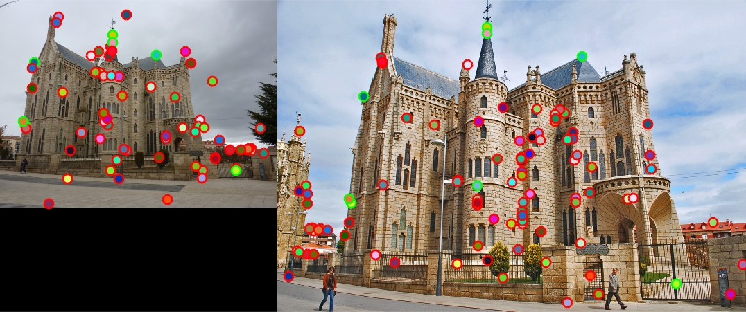
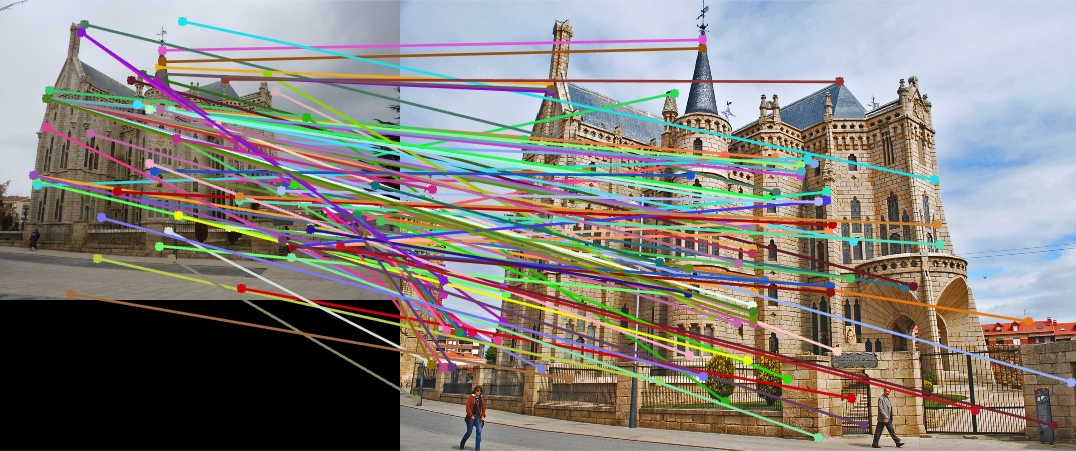
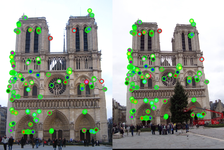
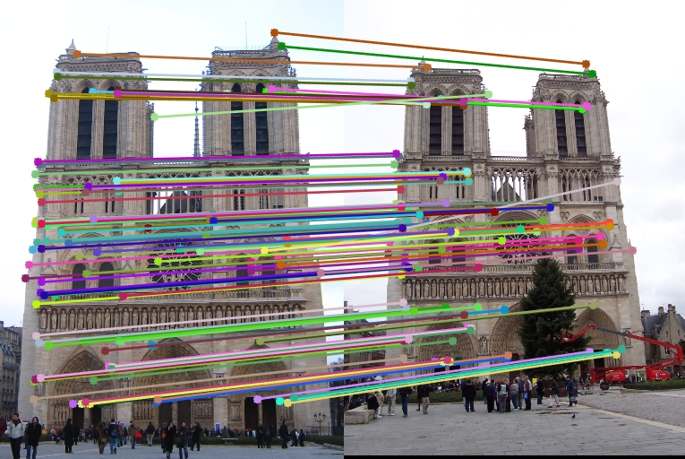
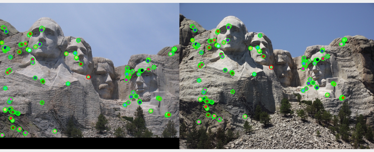
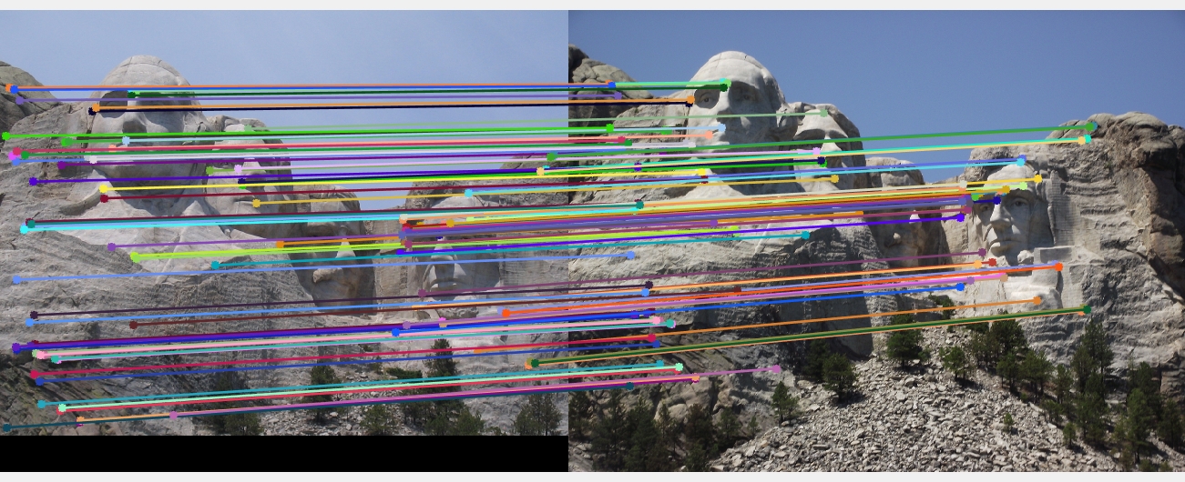
Results of local feature matching run on example images
Notre Dame
Mount Rushmore
Episcopal Gaudi