Project 2: Local Feature Matching
Overview
For the purpose of this project, we were tasked with implementing 3 parts of a feature-matching pipeline for images using a simplified version of SIFT algorithm: get_interest_points, get_features, and match_features. The general idea is to be able to match features of an object using pictures taken of it from different positions/different lighting/etc. Since we were provided with cheat_interest_points function, it proved to make more sense for me to work on the assignment in the opposite order, starting with match_features and ending with get_interest_points.
Implementing match_features
Implementing feature matching was probably the least complex part of the project. Given two matrices filled with vector represenations of features (features1 and features2), the function needs to return two matrices: one with matches of indices of feature vectors from features1 to features2 and another one with confidence score for each match made.
First, I could not assume that both of the input matrices would have the same number of features, so I made sure that the number of output matches is equal to the smaller number of features between features1 and features2. Then, I just simply iterated through the smaller input matrix of features and ran find_match on every feature. find_match is a helper function I wrote that takes in a feature and the matrix filled with all of the features from the other image, and it outputs the best match as well as the nearest-neighbor ratio that serves as an reverse confidence, which is why when we try to sort matches by confidence later on, we do it in the ascending order (i.e., because lower nearest-neighbor ratio indicates a better match). The code for both can be seen below:
function [matches, confidences] = match_features(features1, features2)
    num_features = min(size(features1, 1), size(features2, 1));

    if size(features1, 1) < size(features2, 1)
        smaller_array = features1;
        bigger_array = features2;
    else
        smaller_array = features2;
        bigger_array = features1;
    end

    matches = zeros(num_features, 2);
    confidences = zeros(num_features,1);
    for i=1:num_features
        current_feature = smaller_array(i,:);
        [match, confidence] = find_match(current_feature, bigger_array);
        if size(features1, 1) < size(features2, 1)
            matches(i, :) = [i, match];
        else
            matches(i, :) = [match, i];
        end
        confidences(i) = confidence;
    end

    [confidences, ind] = sort(confidences, 'ascend');
    matches = matches(ind,:);
end
function [match, confidence] = find_match(feature, other_features)
    c1 = Inf(1);
    d1 = Inf(1);
    c2 = Inf(1);
    d2 = Inf(1);
    for i=1:size(other_features,1)
        f = other_features(i, :);
        d = norm(feature - f);
        if (d < d1)
            c2 = c1;
            d2 = d1;
            c1 = i;
            d1 = d;
        elseif d < d2
            c2 = i;
            d2 = d;
        end
    end
    match = c1;
    confidence = d1/d2;
end
After finishing this part, nothing has changed as opposed to random matching, and I still had around 3% correctness on Notre Dame.
Implementing feature extraction
The next step was to actually implement a SIFT-like feature extractor.
First, I implemented a couple of helper function to make my code more organized and thus more debuggable and readable: create_descriptor and group_gradient_dirs. However, before I explain what they do, I will need to provide a high-level explanation of how overall my solution works.
Initially, I retrieve two matrices, one containing gradient magnitudes and the other one containing gradient directions for the input picture, using in-built imgradient function. Then, I do a pre-processing step in order to save some computing time. When I call group_gradient_dirs that I wrote, it takes in the gradient matricies we just retrieved, and for every single pixel, it creates an 8-dimensional vector filled with zeros, and then assigns the magnitude value at that pixel to a particular dimension of that vector depending on which sector of unit circle it falls into (total of 8 sectors). For example, if a pixel has gradient magnitude of 3 and direction of 110deg, then it will be represented as [0;0;0;0;0;0;3;0]. The order of bins is arbitrary, it just has to be consistent throughout the whole run. When the function creates such representation for every pixel, it returns a matrix filled with thse vectors, one for each pixel, with the same dimensions as the original image but with one extra dimension of size 8.
function gradient_dirs = group_gradient_dirs(gd_in, gd_mag)
    gd_out = zeros(size(gd_in, 1), size(gd_in, 2), 8);
    for i=1:size(gd_in, 1)
        for j=1:size(gd_in, 2)
            e = gd_in(i,j);
            if (e > 135)%point between 135 and 180
                gd_out(i, j, 8) = gd_mag(i, j);
            elseif (e > 90)%point between 90 and 135
                gd_out(i, j, 7) = gd_mag(i, j);
            elseif (e > 45)%point between 45 and 90
                gd_out(i, j, 6) = gd_mag(i, j);
            elseif (e > 0)%point between 0 and 45
                gd_out(i, j, 5) = gd_mag(i, j);
            elseif (e > -45)%point between -45 and 0
                gd_out(i, j, 4) = gd_mag(i, j);
            elseif (e > -90)%point between -90 and -45
                gd_out(i, j, 3) = gd_mag(i, j);
            elseif (e > -135)%point between -135 and -90
                gd_out(i, j, 2) = gd_mag(i, j);
            else
                gd_out(i, j, 1) = gd_mag(i, j);
            end
        end
    end
    gradient_dirs = gd_out;
end
Then, I call my create_descriptor function on every single interest point that isn't too close to the edge of the image(i.e., around which it is possible to create a feature of required width without getting out of image bounds). create_descriptor takes in a 16x16x8 (or YxYx8, with Y being the feature width) patch out of the pre-computed array we just obtained and cell width used to know in how many SIFT cells we would need to split our histograms. For every SIFT cell, we sum all the 8-dimensional vectors in the pre-computed matix that lay in the bounds of that cell and add it to a matrix that accumulates histograms for every single SIFT cell. When done, we flatten out the matrix into a 128-dimensional vector and normalize it, which yields the desired feature.
function descriptor = create_descriptor(gd_arr,cell_width)
    vector_arr = zeros(16, 8);
    vector_index = 1;
    for y=1:4:16
        for x=1:4:16
            current_vector = zeros(1,8);
            for i=y:y+cell_width-1
                for j=x:x+cell_width-1
                    current_vector = current_vector + rot90(squeeze(gd_arr(i, j, :)));
                end
            end
            vector_arr(vector_index, :) = current_vector;
            vector_index = vector_index + 1;
        end
    end
    vector_arr = vector_arr(:);
    norm_vector_arr = norm(vector_arr);
    if norm_vector_arr > 0
        vector_arr = vector_arr/norm_vector_arr;
    end
    descriptor = rot90(vector_arr);
end
After we extracted features for every interest point, we return the matrix of all of the features, thus successfully completing our implementation of get_features. At this point, I managed to acquire around 74% accuracy on Notre Dame, 40% on Mount Rushmore, and closer to 7% on Episcopal Gaudi.
function [features] = get_features(image, x, y, feature_width)
    if size(image,3) == 1
        grayscale_img = image;
    else
        grayscale_img = rgb2gray(image);
    end
    pad = feature_width/2;
    [Gmag, Gdir] = imgradient(grayscale_img);

    feature_list = zeros(size(x,1), 128);
    binned_gd = group_gradient_dirs(Gdir, Gmag);
    for i=1:size(x,1)
        if round(x(i))-pad+1 > 0 && round(x(i))+pad <= size(binned_gd,2) ...
					&& round(y(i))-pad+1 > 0 && round(y(i))+pad <= size(binned_gd,1)
            patch = binned_gd(round(y(i))-pad+1:round(y(i))+pad, round(x(i))-pad+1:round(x(i))+pad, :);
            feature_list(i, :) = create_descriptor(patch,feature_width/4);
        end
    end
    features = feature_list;
end
Detecting interest points
function [x, y, confidence, scale, orientation] = get_interest_points(image, feature_width)
    if size(image,3) == 1
        grayscale_img = image;
    else
        grayscale_img = rgb2gray(image);
    end

    w = fspecial('Gaussian', 3, 2);

    [Ix, Iy] = imgradientxy(grayscale_img);
    Ix2 = imfilter(Ix.^2,w);
    Iy2 = imfilter(Iy.^2,w);
    Ixy = imfilter(Ix.*Iy,w);

    a = 0.06;

    H = Ix2.*Iy2 - Ixy.^4 - a*(Ix2+Iy2).^2;
    %prevent features from being on edges
    H(1:feature_width, :) = 0;
    H(size(H,1)-feature_width:size(H,1), :) = 0;
    H(:, 1:feature_width) = 0;
    H(:, size(H,2)-feature_width:size(H,2)) = 0;

    threshold = mean2(H);
    H = H.*(H > threshold*max(max(H)));

    x = [];
    y = [];
    nmsupp = colfilt(H, [8 8], 'sliding', @max);
    H = H.*(H==nmsupp);
    [yl, xl] = find(H);

    x = [x;xl];
    y = [y;yl];
end
To detect interest points, I utilized Harris corner detection algorithm. First, I created a Gaussian filter with size 3 and sigma equal to 2. Then, I found matrices Ix and Iy using in-built imgradientxy and found Ix2/Iy2/Ixy (needed for the Harris algorithm) by running imfilter using the earlier created Gaussian filter and member-wise squares of the matrix (for Ix2 and Iy2) or member-wise multiplication of them (Ixy). Then I simply ran the Harris algorithm with alpha being 0.06 to obtain matrix H. Then I eliminated interest points close to the edge by nullyfing entries in the matrix corresponding to them. After that, I eliminated any interest points whose value was less than the threshold (which I assigned to be the mean of all values in H) and implemented a non-maximum suppresion algorithm using a sliding window. I tried to vary size of the sliding window in orderd to find the sweet spot of time and performance (the following tests were performed on Notre Dame picture). With a 16x16 window, I managed to get up to 72% correct matches with the runtime of less than a minute.
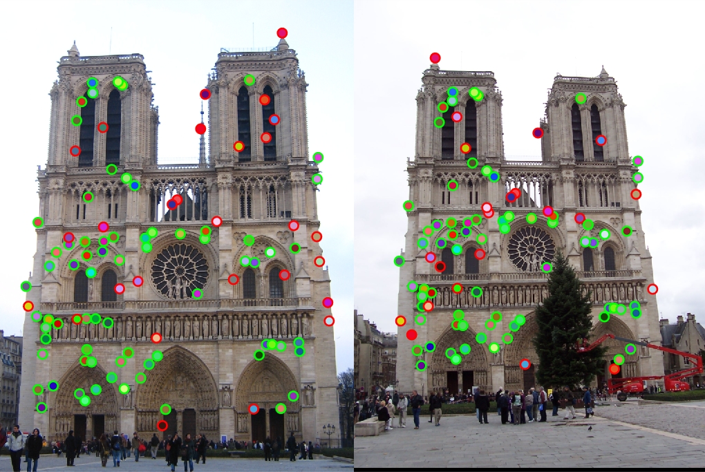
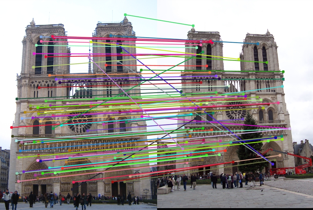
Changing it to 8x8 gave me a runtime of slightly more than a minute with 94% accuracy (which is an extreme improvement).
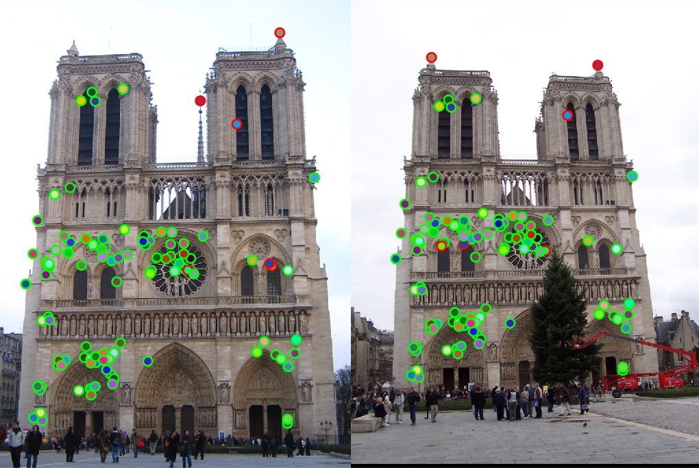
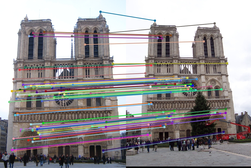
Making the window 3x3, I got some more accuracy, but at the expense of running time of more than 10 minutes.
A smaller window means more interest points, and it proved to give me better results than using a 16x16 one. However, I decided that 8x8 provided a good balance between runtime and accuracy as opposed to 3x3 that only slightly increased it, so in the end, I left it at 8x8. To conclude the implementation, I simply returned coordinates of every non-zero value in the resulting matrix. As the last suggested improvement, I limited the list of feature pairs only to the 100 most confident ones. As can be seen, changing the radius of non-maximum suppression (i.e., the size of sliding window) can have a very profound effect on the accuracy, but then a balance between reasonable runtime and extra accuracy gain is needed.
It isn't over (yet)
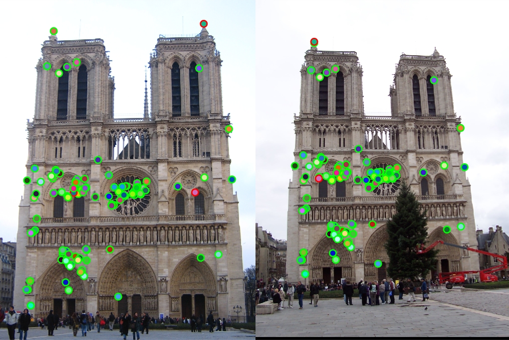
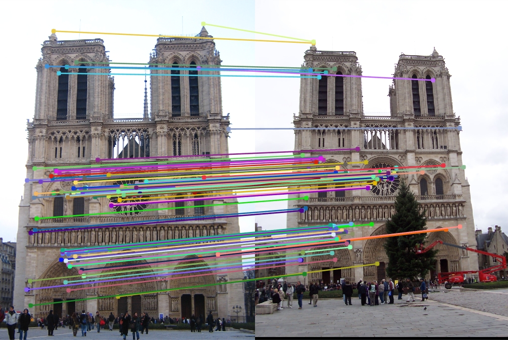
As suggested, I decided to modify proj2.m in order to get better results. A significant improvement in performance came from limiting the number of feature matches to only the 100 most confident ones, which makes sense since low-confidence matches are probably not that good.
After experimenting in the paragraph above to see the most optimum configuration for Notre Dame, I decided to run the configuration with the highest accuracy (3x3 window) on other 2 picture sets just to see what is the maximum accuracy I can push out for them.
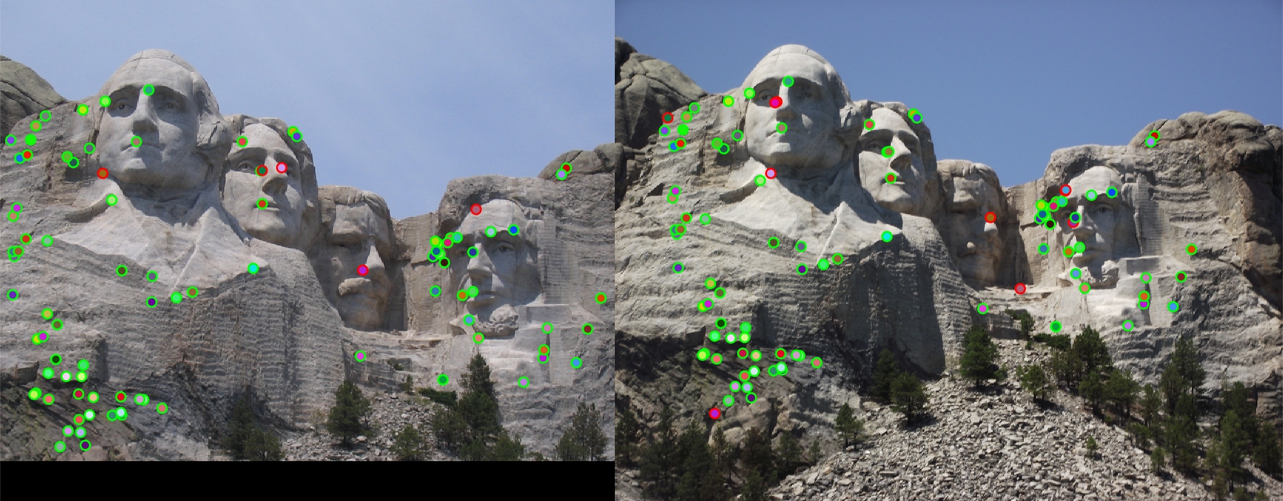
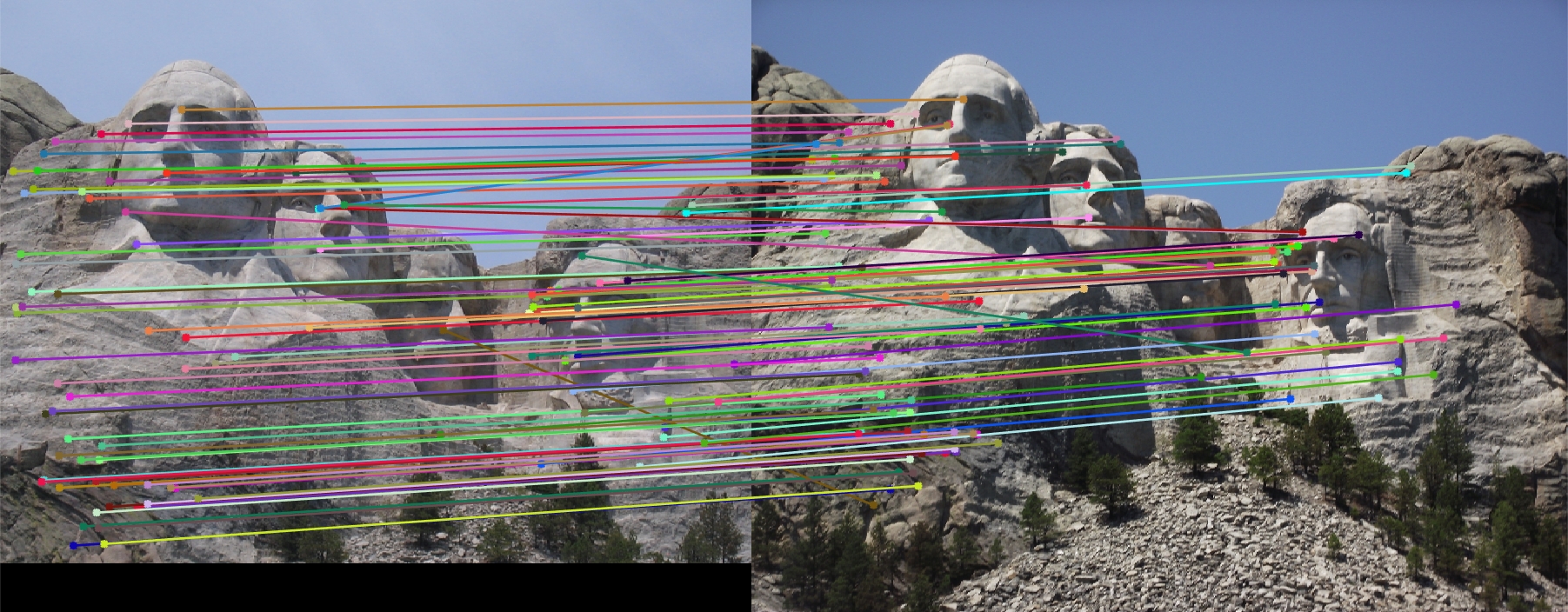
For Rushmore, we obtained fairly good results (90%), since the only extra challenge it presented, as opposed to Notre Dame, very stark lighting difference.
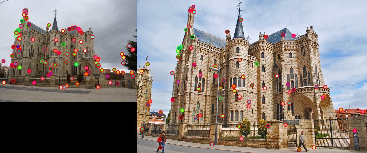
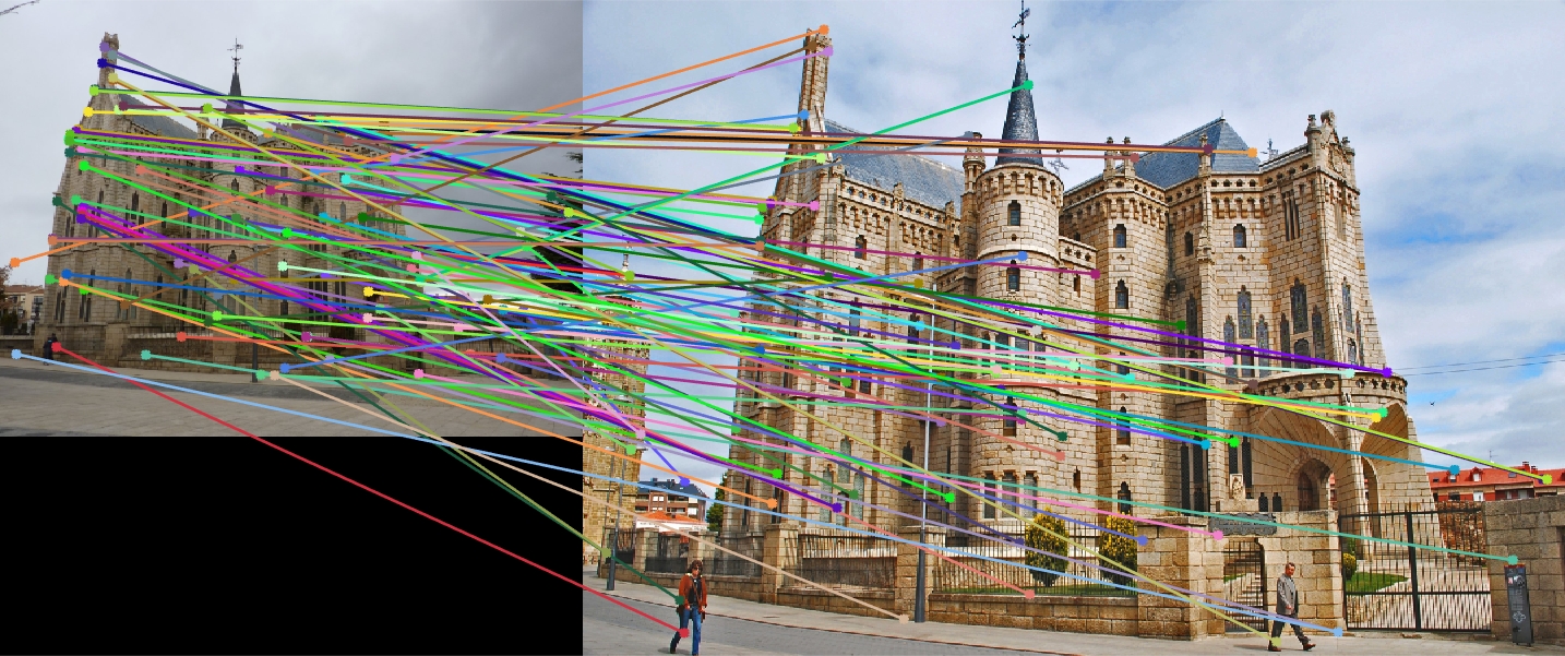
For Gaudi, arguably the most difficult picture pair, the maximum accuracy I was able to reach was 12%. I can attribute this to radical differences in scale, lighting, angle of the images, and a number of things (people, extra tower to the left, trees to the right) that are present in one image but not the other that can easily be identified as features. Notre Dame has people as well, but they are presented in similar quantities and positions in both pictures in the pair, as well as being mostly clumped into crowds, as opposed to singular people.