Project 2: Local Feature Matching
All that's missing is the hunchback.
For this project, we were tasked with creating a local feature matching algorithm as described in secton 4.1 of our Szeliski textbook. This algorithm would follow a simplified version of the SIFT pipeline, and would be able to match different views of the same scene.
Matching Algorithm
The matching algorithm could be split into 3 parts:
- Finding interest points
- Finding features within the interest points
- Matching features across images
Finding Interest Points
For this project, I implemented a Harris Corner Detector by following Algorithm 4.1 in section 4.1.1 in the textbook. Once the detector was created I supressed the edges to avoid stray interest points that were not within the main focal point of the image. I simply did this by setting everything that was not within the feature_width of the Harris Detector to 0, so that the pixels were black. After this I set a threshold to determine what values in the detector were actually Harris Corners. Finally, I used the colfilt method to supress any values that werent max values (non-maximum supression), so as to only have the highest interest points.
Finding Features
Finding features was by far the most difficult part of this project. SIFT is a somewhat convoluted (no pun intended) process that was difficult to understand. In its simplest form, SIFT creates a frame around each interest point, then divides those frames into 16 cells (4 x 4 grid), and computes a gradient histogram for each cell in 8 dimensions. This creates a feature set with 128 (4 x 4 x 8) dimensions. The way I was able to implement the SIFT algorithm required me to nest a series of for loops within one another, so it is definitely a bottleneck in the processing of these images. Although I do believe there is some way to optimize this process, my lack of familiarity with MATLAB stopped me from figuring out another successful method. Overall, I was still pleased with how my implementation worked, as it provided a reasonable amount of features that could be matched by the next step.
Matching Features
Matching features was the easiest portion of this project by far. I simply implemented the Ratio Test equation that was shown in equation 4.18 in our textbook, then tested different distance thresholds until I was satisfied with the matching alogrithm's accuracy. For the images used to test, I was able to get the best accuracy with a distance threshold of 0.7, as values higher or lower than this reduced accuracy, or provided too few points that were matches, potentially allowing two images of somewhat similar features to be matched.
General Comments
Overall, I am satisfied with my success on this project as I was able to build up my accuracy along similar expected growth on the main Notre Dame image set as Professor Hayes outlined in the project outline. I enjoyed working with the feature matching and interest point detection of this project, but the confusing process that is SIFT was quite frustrating to try to implement, and I probably could have done it better.
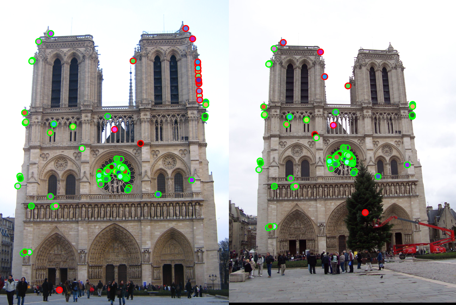
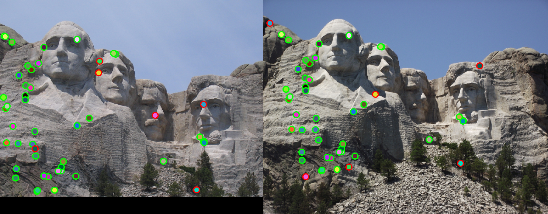
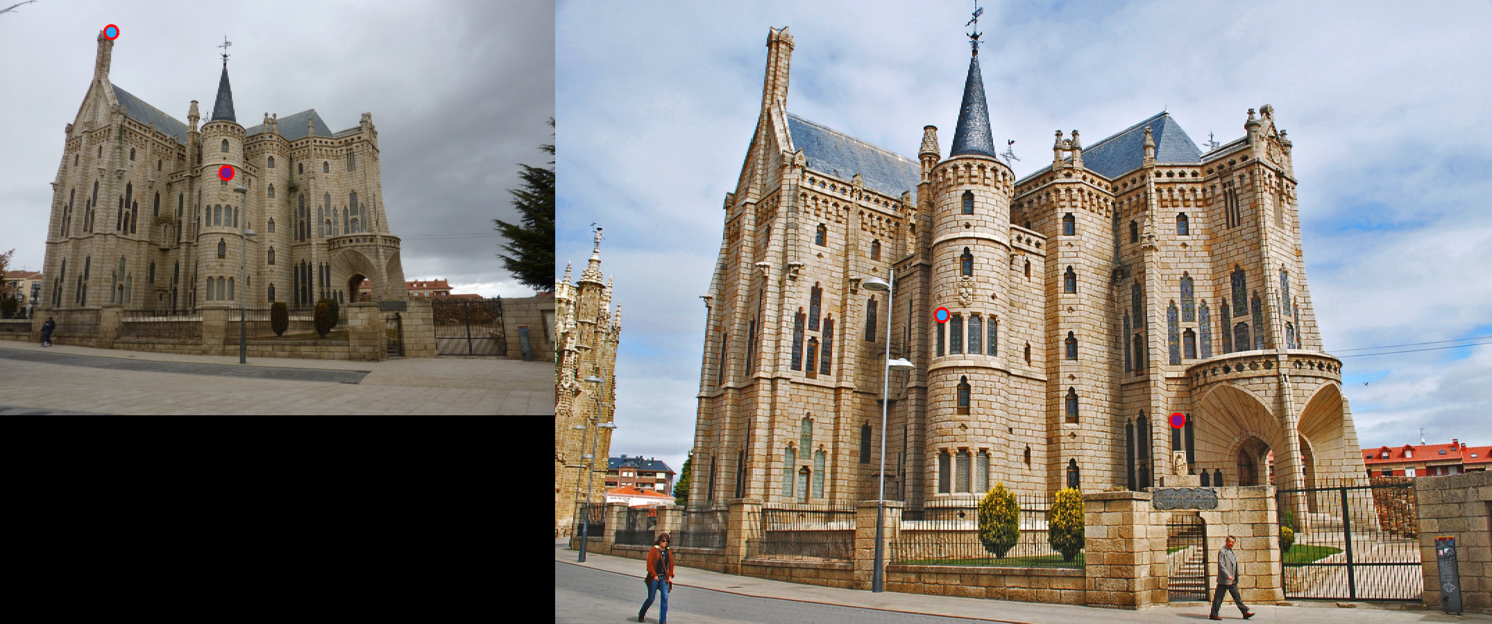
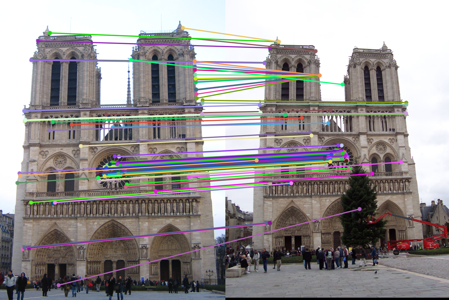
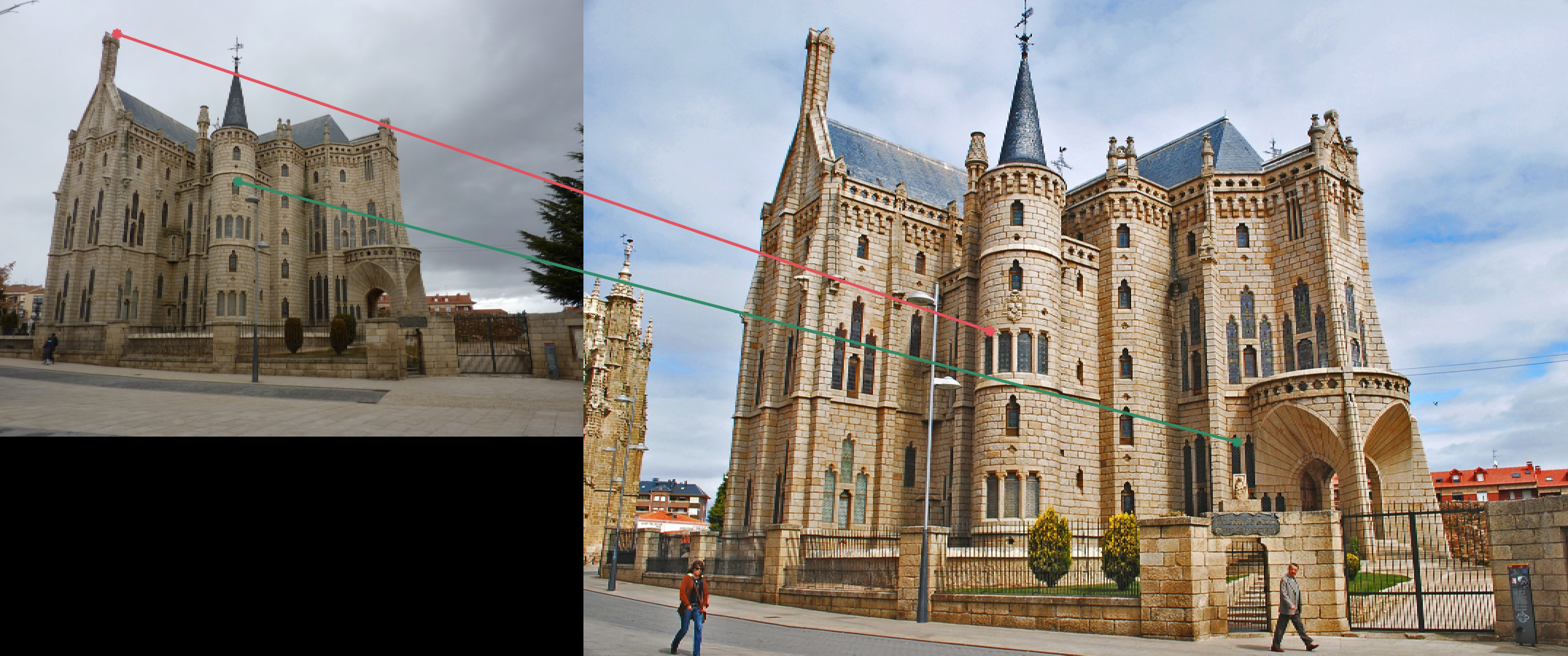
Results
The following are my results from each 3 sets of images. As you can clearly see, my code failed quite miserably on the Epsicopal Gaudi images, but did well on the other 2 sets.
|

|