Computer Vision Project

1 Introduction

This report discusses the implementation details and success rate of the feature identification and extraction assignment for CS6476. In particular, this assignment involes utilizing a Harris corner detector to identify interest points, extracting the features with a SIFT-like technique, and matching these designated features between two separate images. To show the validity of our results, we show the success rate of this feature detection and matching. Furthermore, we demonsrate the improments of the graduate credit requirements.

2 Detecting Interest Points

This section discusses the implementation of the Harris corner detector, extraction of interest poings, and non-maximal supression.

2.1 Harris Corner Detector

The Harris corner detector is a tool for identifying important points in an image. This techniques utilizes the image gradients to distinguish corners in the image. Generally speaking, one quadratically approximates an intensity function with a two-dimensional Taylor expansion. This quadratic approximation is
$xTM x,$ (1)

where x = [uv] ^T are pixel coordinates, and M is
$[ 2 ] Ix Ixy2 . Ixy Iy$ (2)

M tells us likely a particular point is to be a corner through the following function
$2 R = detM − αTr(M ) ,$ (3)

where α is a weighting parameter that is typically defined to be 0.04. Eqn. 3 provides a tool to detect corners. If R > 0, the value is typically a corner, though some thresholding is normally applied.

2.2 Connected-Component Thresholding

Due to the thresholding of Eqn. 3 for the detection of corners, the Harris algorithm generates many interest points. In order to prune these points to prevent large processing overhead, a black and white image is formed. Each index of this black and white image is defined by
${ 1 if Rij > T aij = 0 o.w. ,$ (4)

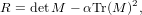
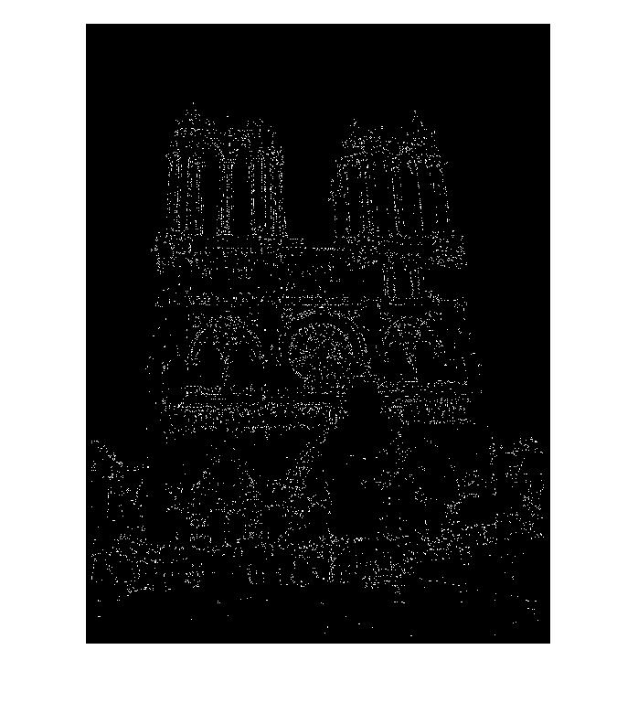
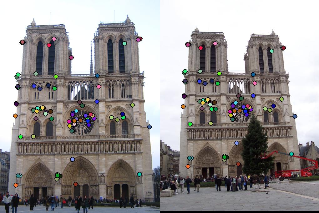
where T > 0 is some threshold. Let I_b = [a_ij] be the binary image. Utilizing MATLAB’s ”bwconncomp” function, the connected components of this image are formed. From each component, the point that maximizes Eqn. 3 is selected. Fig. 1 shows the results of this interest point detection algorithm on the Notre Dame image.

Figure 1: Retrieved interest points using Harris detector and connected component max algorithm. This method can suppress relatively important interest points through the maximization process, leading to a sparse feature space.

2.3 Nonmaximal Suppression (Grad. Credit)

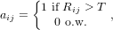
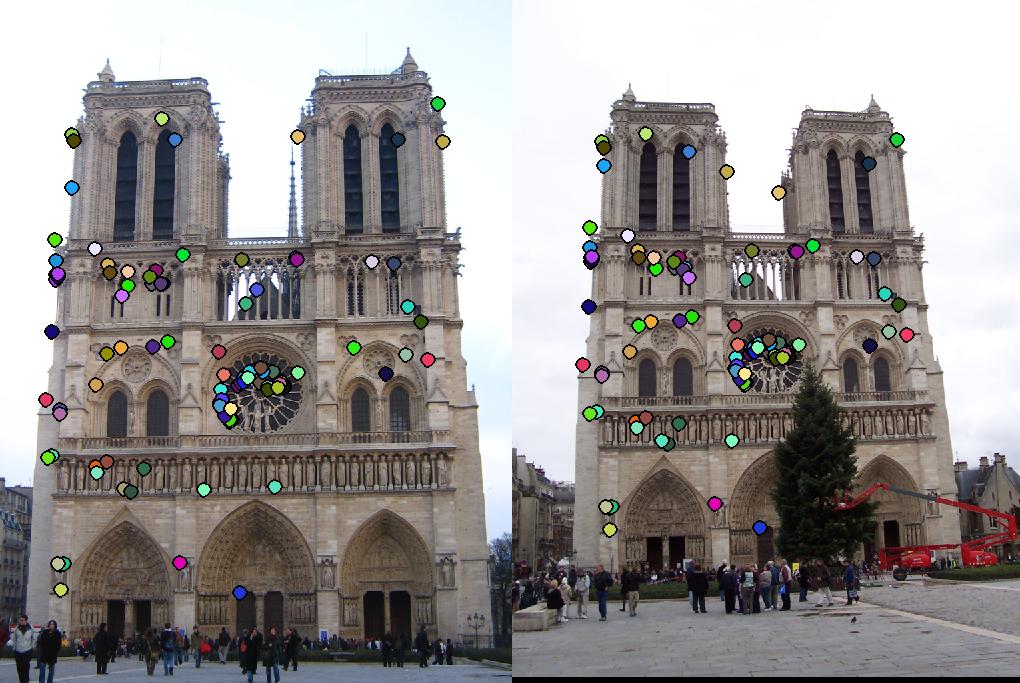
Taking the maximum in every connected component can arbitrarily discard relatively good interest points. To address this issue, we apply a nonmaximal suppression technique. In particular, for each connected component, we retrieve the first N local maxima, where N is a positive integer. This technique allows us to retrieve the best interest points, without sacrificing performance. Furthermore, it causes more overlap between the feature sets for each image, making the matching process more reliable in the last step of this project. Fig. 2.3 shows the improved detection method for these interest points on the supplied Notre Dame image pair.

Figure 2: Detected interest points with the nonmaximal suppression technique. This technique ensures that interest points are evenly spatially distributed. Compared to the usual connected component max algorithm, this method generates more dense feature sets around highly influential areas, aiding the matching process.

3 Feature Extraction

Given a set of interest points, the next stage in the image-matching pipeline is to extract SIFT-like features from the image. Given an interest point, our SIFT-like features extract the image gradient magnitude and direction for 8 direction in a 16x16 box surrounding each interest point. In particular, each 4x4 section of the 16x16 feature box contributes an image magnitude and gradient in 8 directions, for a total of 128 features.

3.1 SIFT

This method takes advantage of the Derivative of Gaussian (DoG) filtering process. Let g be the image in question and h be a filter. The application of h to g is a convolution process designated by
$f = g ∗h.$ (5)

Given that f is a filtered image, the gradient is given by
$-∂-[g ∗h] = g ∗-∂-h, ∂x ∂x$ (6)

by the associativity property of the convolution operator. Thus, it is only required to convole the image g with a DoG filter. One benefit of the DoG filter is that it is steerable. That is, an oriented filter (i.e., a filter rotated by some amount θ) can be represented by
$hθ = cos(θ)∂xhx + sin(θ)∂yhy.$ (7)

Utilizing this property, we compute the magnitude of the gradient in direction θ by using an oriented filter h_θ. Thus, the image is convolved with 8 separate oriented filters, producing 128 features.

By utilizing SIFT-like features, rather than the naive 16x16 average, the accuracy of the matching process went from 66% to 90%.

3.2 Principal Component Analysis (Grad. Credit)

Because the SIFT-like feature extraction process generates very high-dimensional features, we reduce the dimensionality of the feature vector by applying a Principal Component Analysis (PCA). PCA is typically performed over many images to achieve high confidence in the dimensionality reduction. However, in this case, we only receive two images. Thus, we perform the following steps

Detect interest points
Extract features for each image
Combine both sets of features into one 2n × k vector
Perform PCA on the combined feature vector
Take the first N feature dimensions
Separate into individual n × k − N vectors

Our PCA allowed us to effectively reduce the dimensions of the features to 80 from 128, without a noticable loss in accuracy.

PCA accomplishes dimensionality reduction by performing a change of basis to a covariance representation of the feature vector. From this perspective, a Singular Value Decomposition (SVD) is peformed on the matrix, and the largest singular values are extracted. Thus, the larger the singular value, the more it affects the covariance, implying that the feature is ”important.” Thus, we take the first N of the largest singular values and transform this representation back into the original feature space.

Because this transformation is performed on the entire set of extracted features simultaneously, the ordering of features, relative to each image, is maintained; and consistent results are achieved.

4 Feature Matching

The final component of this feature-matching pipeline is to match each feature from the individual set of features. That is, we must determine the correspondence between the extracted feature sets.

4.1 Ratio Test and Nearest-Neighbor Matching

Initially, we complete this task through a nearest-neighbor search and the ratio test. If we let N₁,N₂ represent the first and second, respectively, neighbors from matching some feature in the first image to another feature in the second image; then, the confidence in this match is given by the ratio test
$N1- N2 .$ (8)

The meaning of this equation is straight-forward: If the ratio is small, then the first feature more closely matches the selected feature than any other feature available. If this result is close to 1, then the matching is ambiguous. That is, the first feature is equally close to many features in the second feature set.

Because the interest point detection algorithm generates many points, we take only the first 100 best-matched features (i.e., features where the ratio test is smallest).

One downside of this matching process is that the naive implementaiton of a nearest neighbor search takes O(n²) time for matching between the two feature sets. To sort 8100 pairs of features, this algorithm took 250s.

4.2 KD Trees (Grad. Credit)

To accelerate the matching process, we implemented a KD-tree data structure and a nearest neighbor search using KD-trees. These implmentation files may be found under ”kd-tree.m” and ”kd-tree-nns.m.” Though we successfully implemented this data structure, we utilized MATLAB’s built-in KD-tree, due to its optimized performance qualities.

Utilizing the KD tree, the same matching process on 8100 features took approximately 35 s with no decrease in accuracy, making the image processing pipieline much faster.

5 Results

This section contains results for the base requirements and the imeplemented graduate course enhancements. In particular, we wish to draw attention to the following areas

Feature extraction
Speed
Accuracy

For each implementation, we present the three given pairs of images, the accuracy of the matching process, and the speed at which the matching was completed. For every other component (e.g., feature extraction), this time remained roughly the same.

5.1 Base Requirements

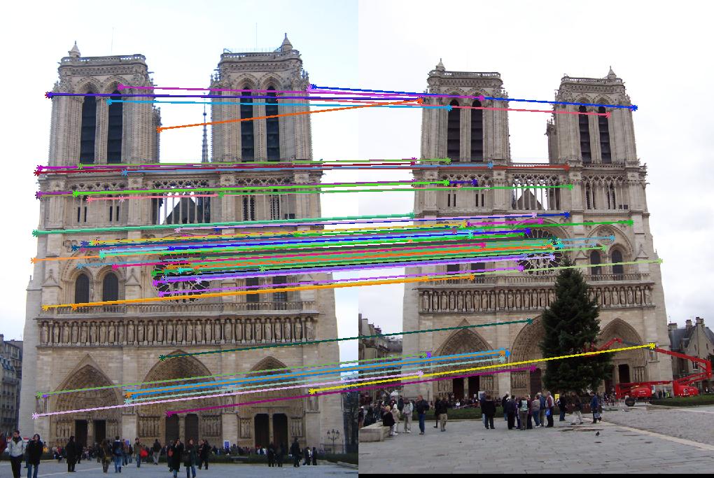
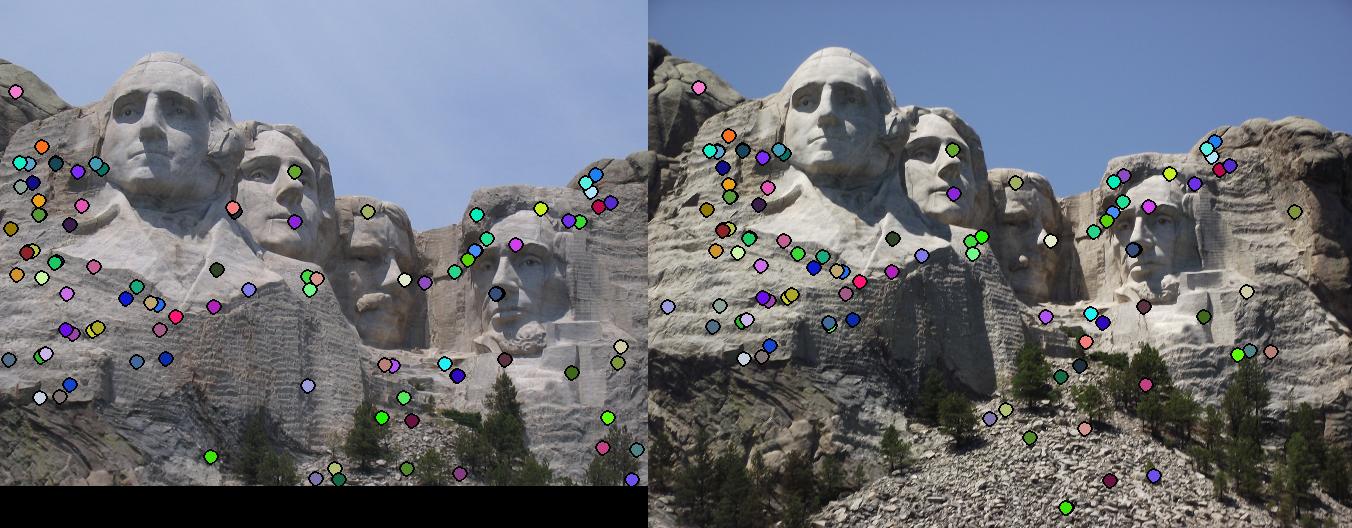
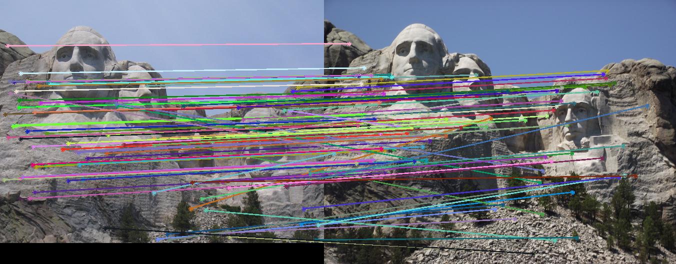
This section contains the results of the image-processing pipeline with only implementations for the base, undergraduate requirements. Figs. 3,4,5 show the results for the baseline implementation. While the accuracy of this approach remained high for the Notre Dame and Mount Rushmore pairs, the processing time became largely prohibitive.

Figure 3: Displays selected features and matches for the Notre Dame pair for baseline requirements. There were 2000 features which took 25 s to match with 91% accuracy.

Figure 4: Displays selected features and matches for the Mount Rushmore pair for baseline requirements. There were 6800 features which took 512 s to match with 98% accuracy.

Figure 5: Displays selected features and matches for the Episcopal Gaudi pair for graduate requirements. There were 6000 features which took 450 s to match with 6% accuracy.

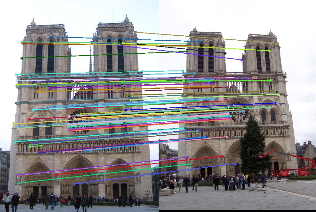
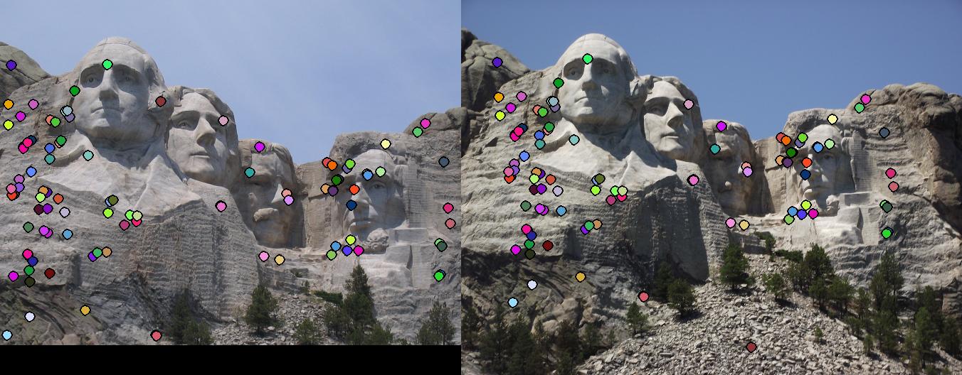
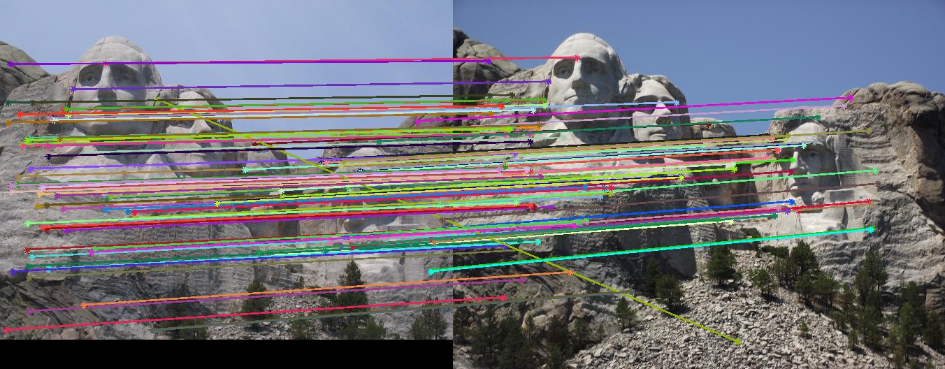
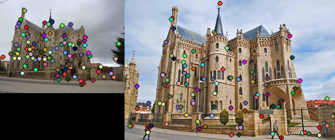
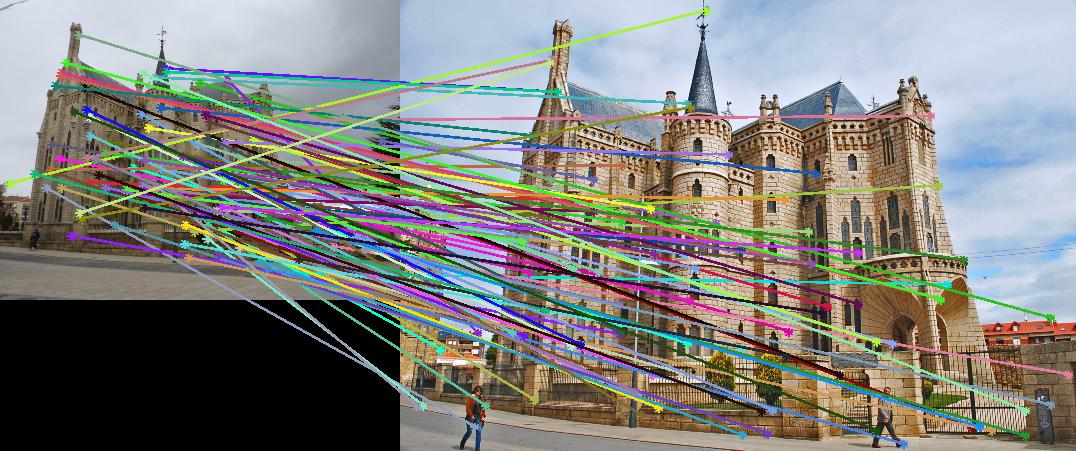
As evidenced by the supplied figures, the modification for the graduate credit requirements vastly increased the speed at which these algorithms ran, allowing for many more features to be examined. Futhermore, the PCA of the features reduced the feature dimensionality by half (i.e., to 64 dimensions). Again, this improvement increased the speed and only slightly decreased the accuracy. Figs. 6,7 show the results of this imlementation. Note that the largest overall gain with this implementation is the acceleration of the nearest-neighbor matching. Additionally, we have omitted the Episcopal Gaudi results due to matching similarity. However, the matching rate remained greatly accelerated with this pair as well.

Figure 6: Displays selected features and matches for the Notre Dame pair for graduate requirements. There were 12000 features which took 54 s to match with 94% accuracy.

Figure 7: Displays selected features and matches the for Mount Rushmore pair for baseline requirements. There were 9100 features which took 143 s to match with 81% accuracy.

6 Conclusions

In this assignment, we discussed and implemented a SIFT-like feature pipieline to retrieve interest points, extract features, and match the features in two distinct images. For the baseline implementation, we utilized a connected component max, brute-force nearest neighbor algorithm, and full feature dimensionality. This approach resulted in prohibitively large run times. By satisfying the graduate credit requirements for this assignment, we were able to greatly improved the run times through usage of KD-trees and dimensionality reduction through a PCA on the extracted features.

Paul Glotfelter