Project 2: Local Feature Matching
On Jan 5, 2004, Andrew Lowe published a paper titled 'Distinctive Image Features from Scale-Invariant Keypoints', which better came to be known as the SIFT paper, a paper that would go on to be cited more than 36,000 times and that propelled him to fame in the community of Computer Vision researchers. Today, we will try to recreate his work on pairs of images.
The SIFT pipiline is composed of three parts,
- Interest Point Detection Finding points that can be matched between two images. Usually 'corner points', determined by a high change in gradient in both directions are easy to match. Hence, we will usually implement some form of corner point detector.
- Local Feature Description A way of succintly describing the points at the corner that is reasonably independent of the image
- Feature Matching A way of finding image descriptors that are close to one another, whre close is defined as correspoinding to the same interest point.
We will code and run an approximation of the SIFT algorithm and display results on the Notre Dame, Mount Rushmore and Episcopal Gaudi image pairs. The pipeline comsists of a Harris corner detector, a 128 bit SIFT like descriptor constructed using a histogram of image patches and a feature matcher that uses euclidean distance to find the close features.
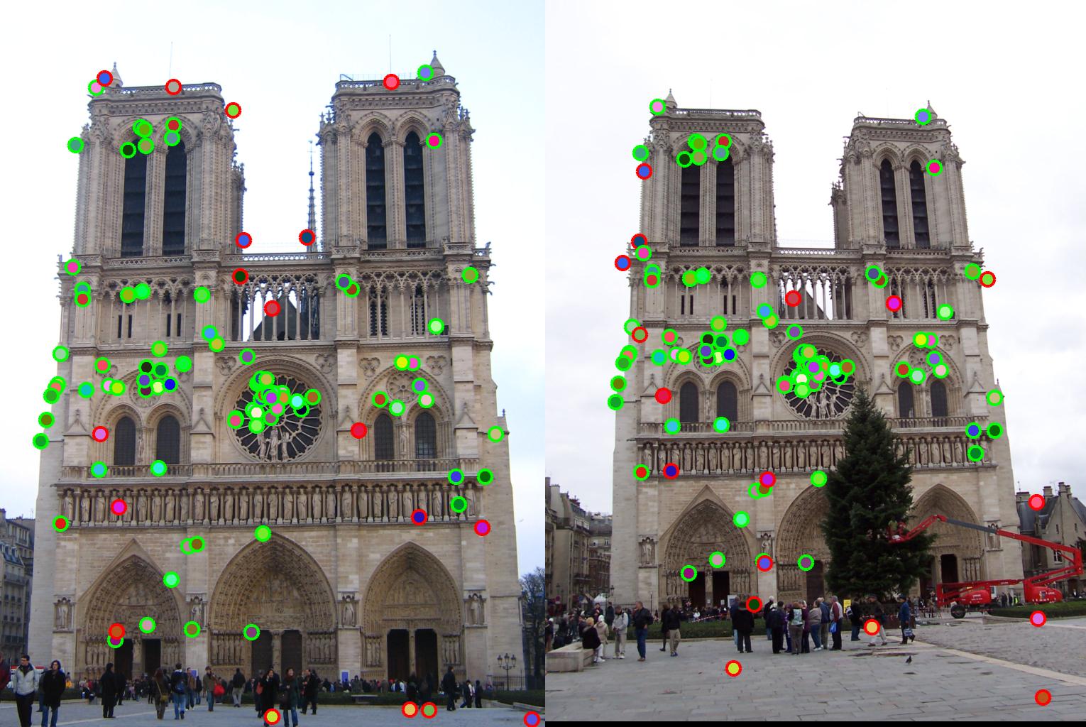
Notre Dame
The Notre Dame example consists of the following pairs of images,
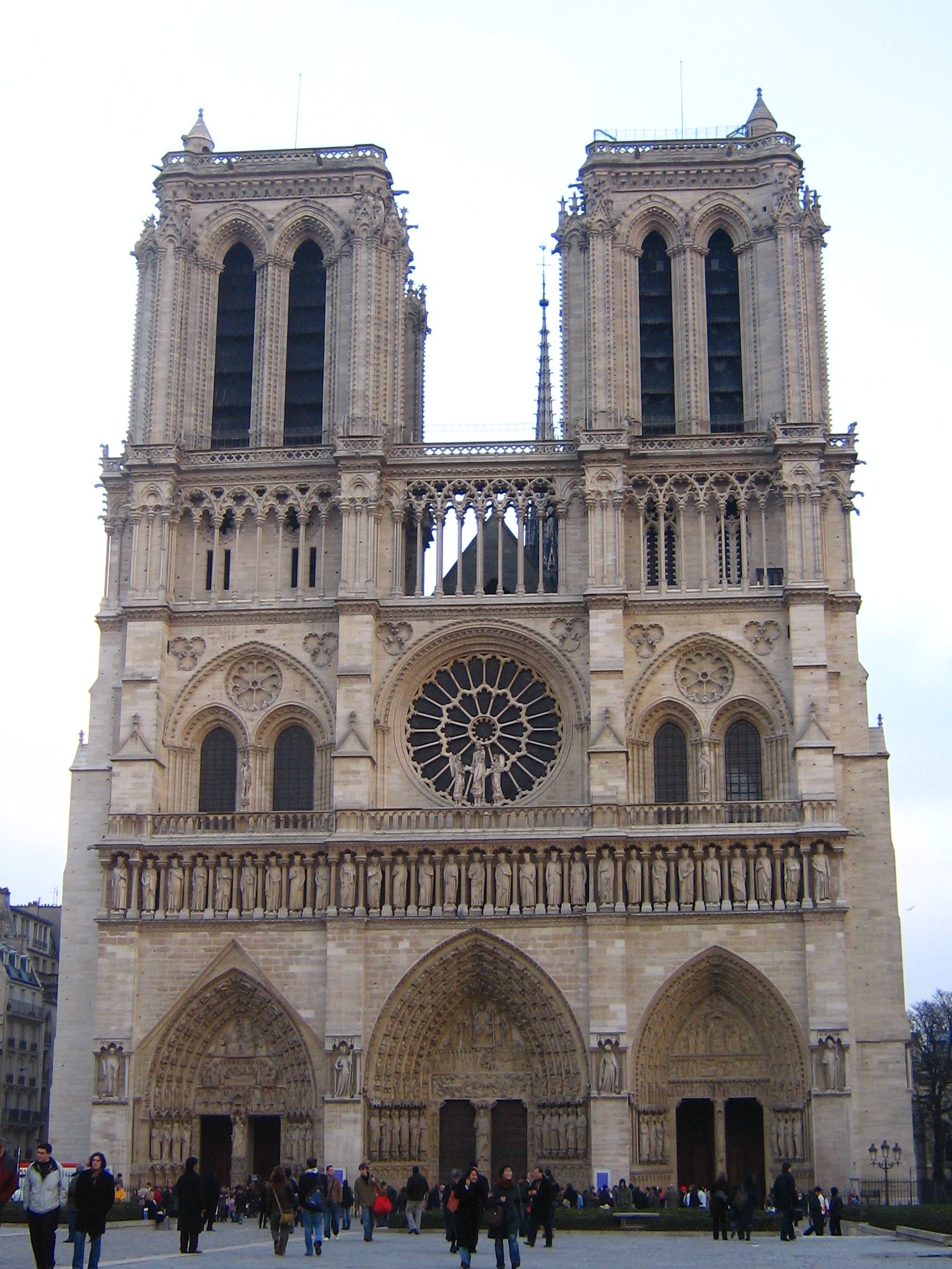
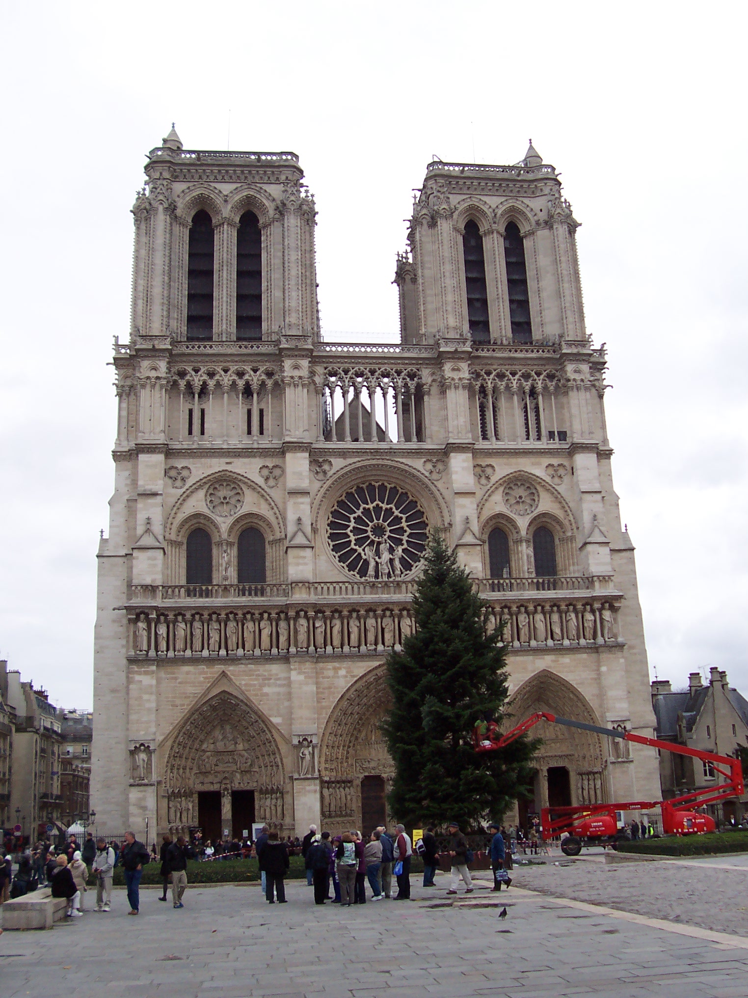
Both images are taken at the same location and have the same subject but are slightly different in orientation, scale, illumination, etc. We run the image pair through our pipeline and obtain the following results.
The interest points obtained by our Harris detector are as follows,
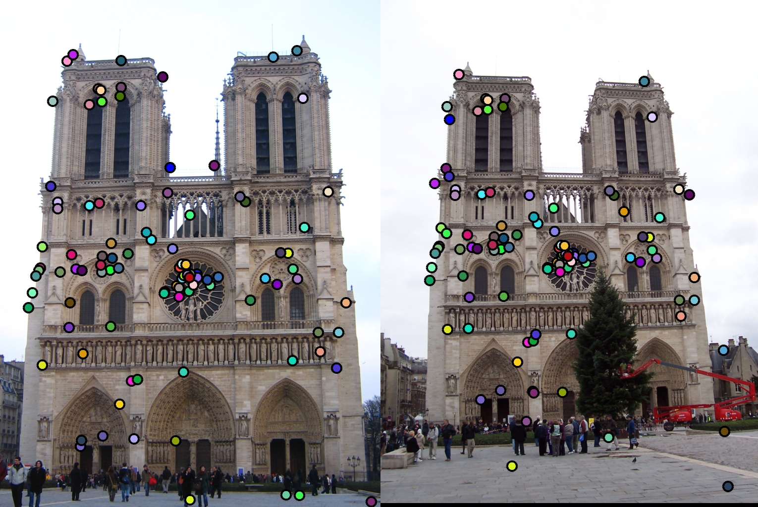
The interest points are obtained at points of sharp change in gradient and not on the smooth part of the image. Note that these are a sample of the interest points obtained by our detector and not the entire set.
Now we will look at the matches that our algorithm comes up with for the pair of images.
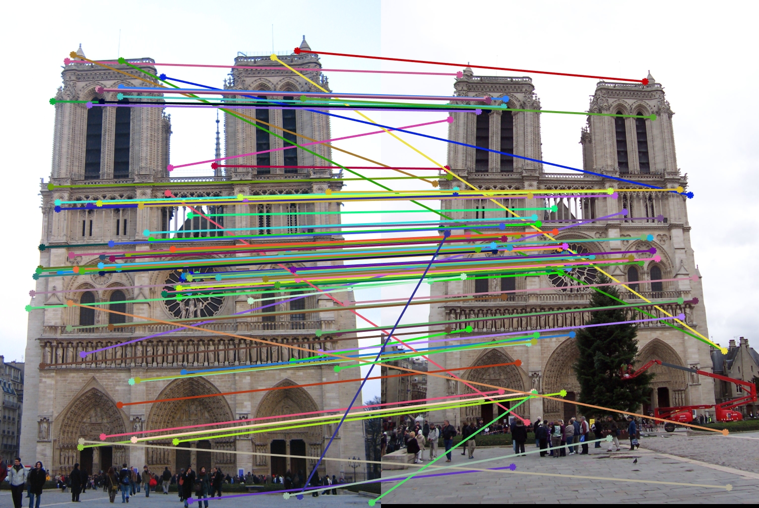
Most arrows go to points that are in the sameplace, though we do observe some strays. The strays represent places the algorithm has failed to build a good enough descriptor that can be deteccted later. The accuracy is 82%. The correct and incorrectly matched points are shown below.
We will now run the algorithm on the Mount Rushmore and Episcopal Gaudi pairs of images.
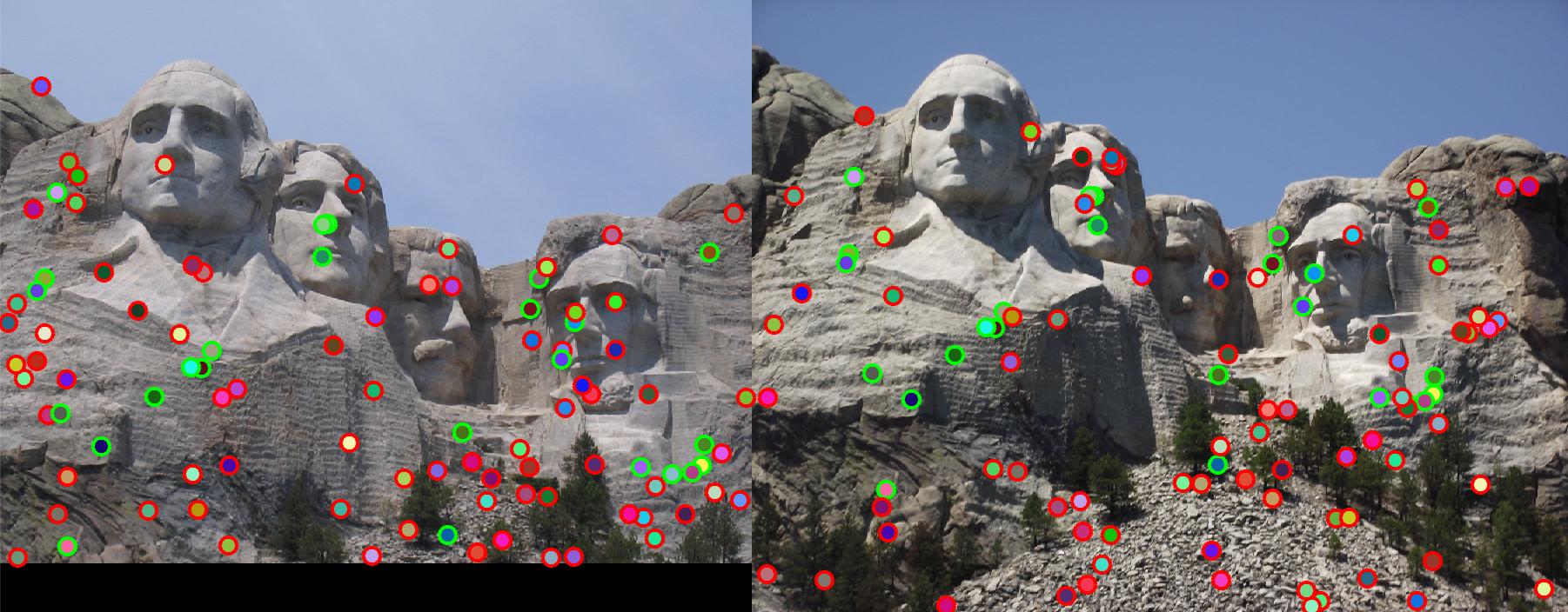
Mount Rushmore
The Mount Rushmore example consists of the following pairs of images,
The interest points obtained by our Harris detector are as follows,
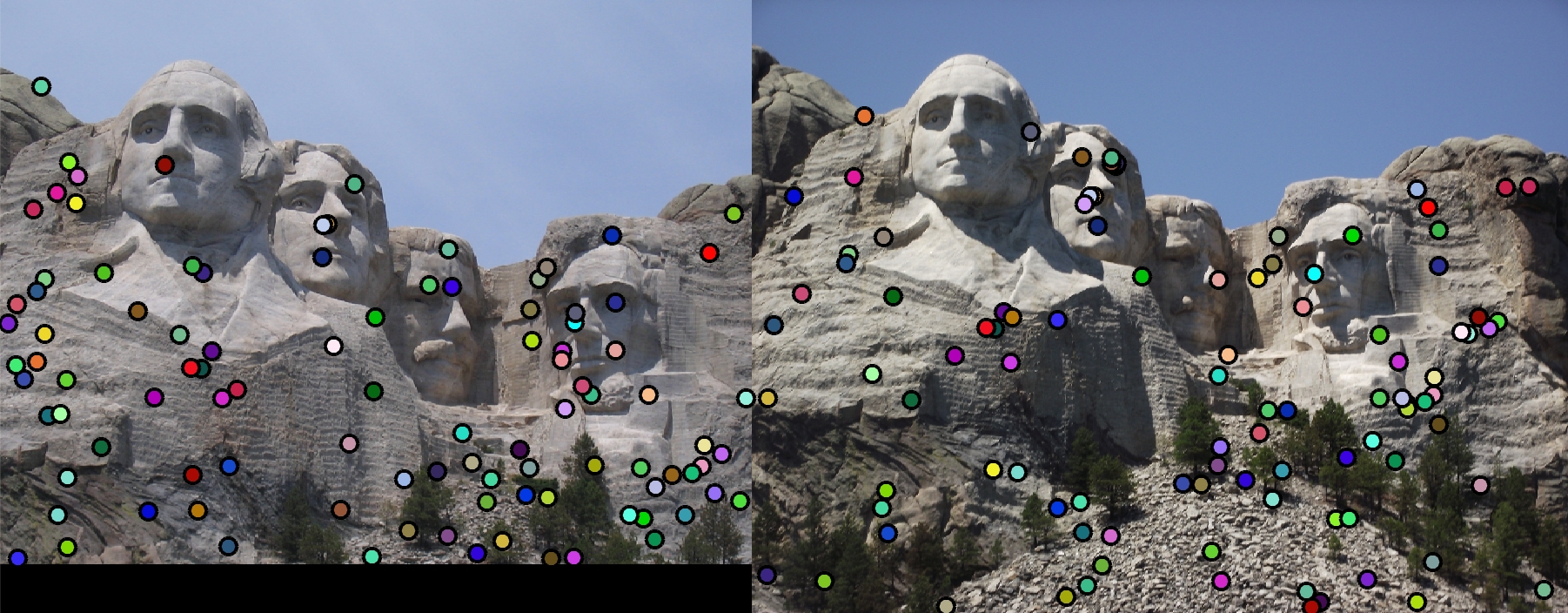
The interest points are obtained at points of sharp change in gradient and not on the smooth part of the image. Note that these are a sample of the interest points obtained by our detector and not the entire set.
Now we will look at the matches that our algorithm comes up with for the pair of images.
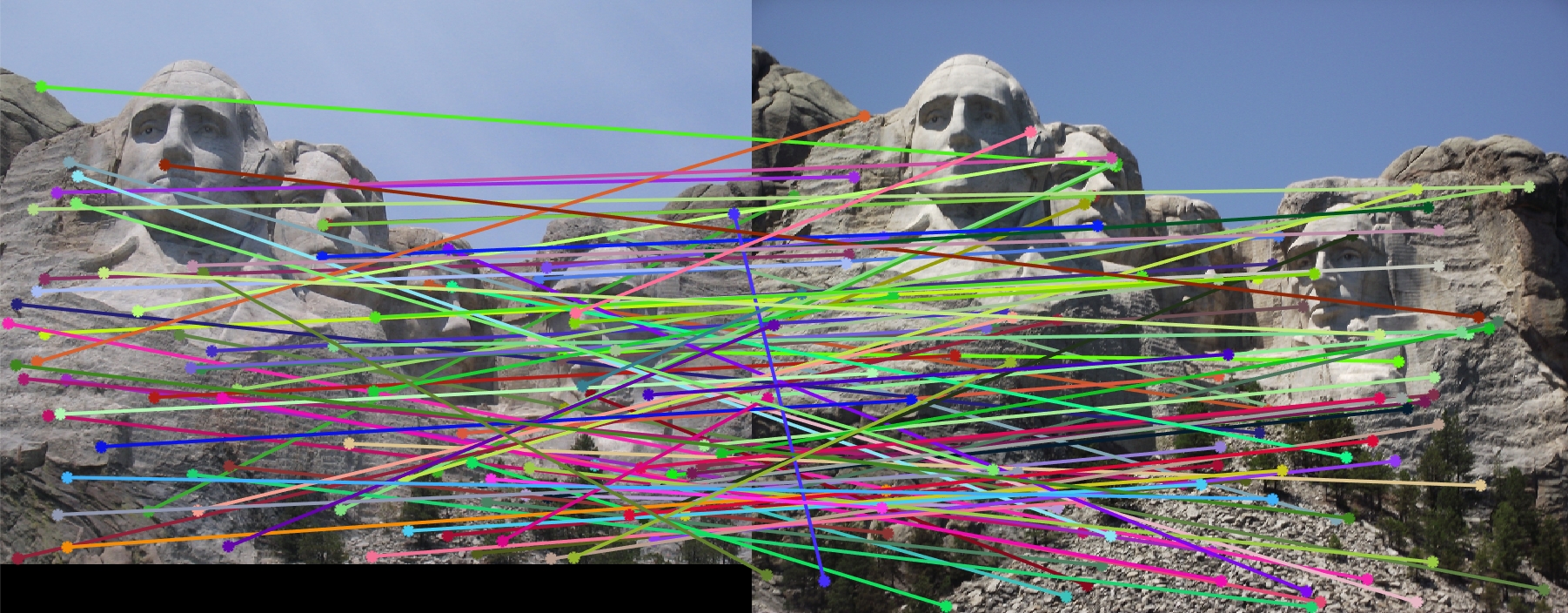
Most arrows go to points that are in the sameplace, though we do observe some strays. The strays represent places the algorithm has failed to build a good enough descriptor that can be deteccted later. The accuracy is 25%. The correct and incorrectly matched points are shown below.
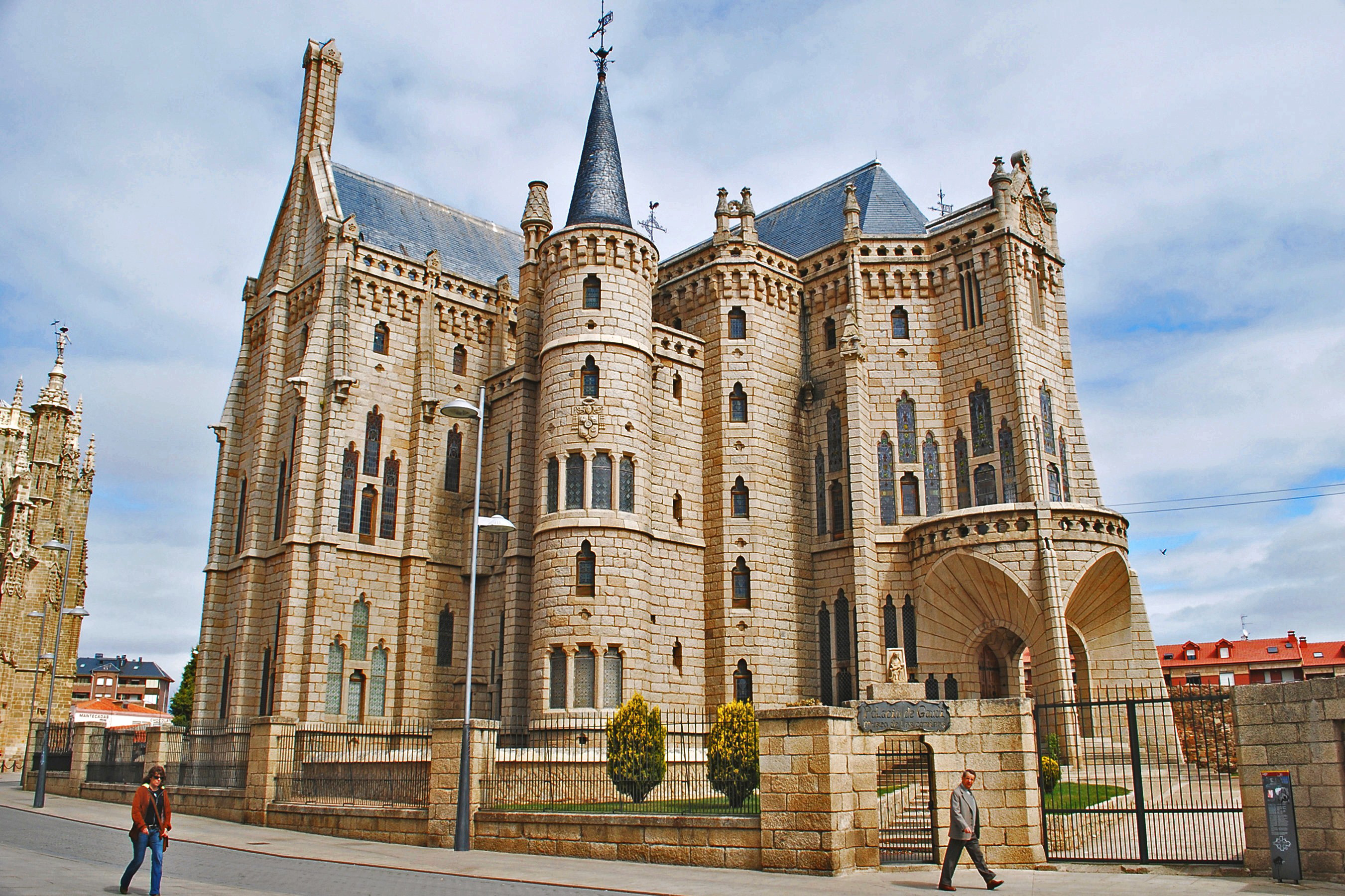
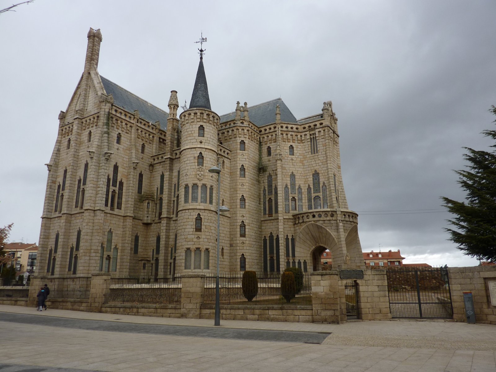
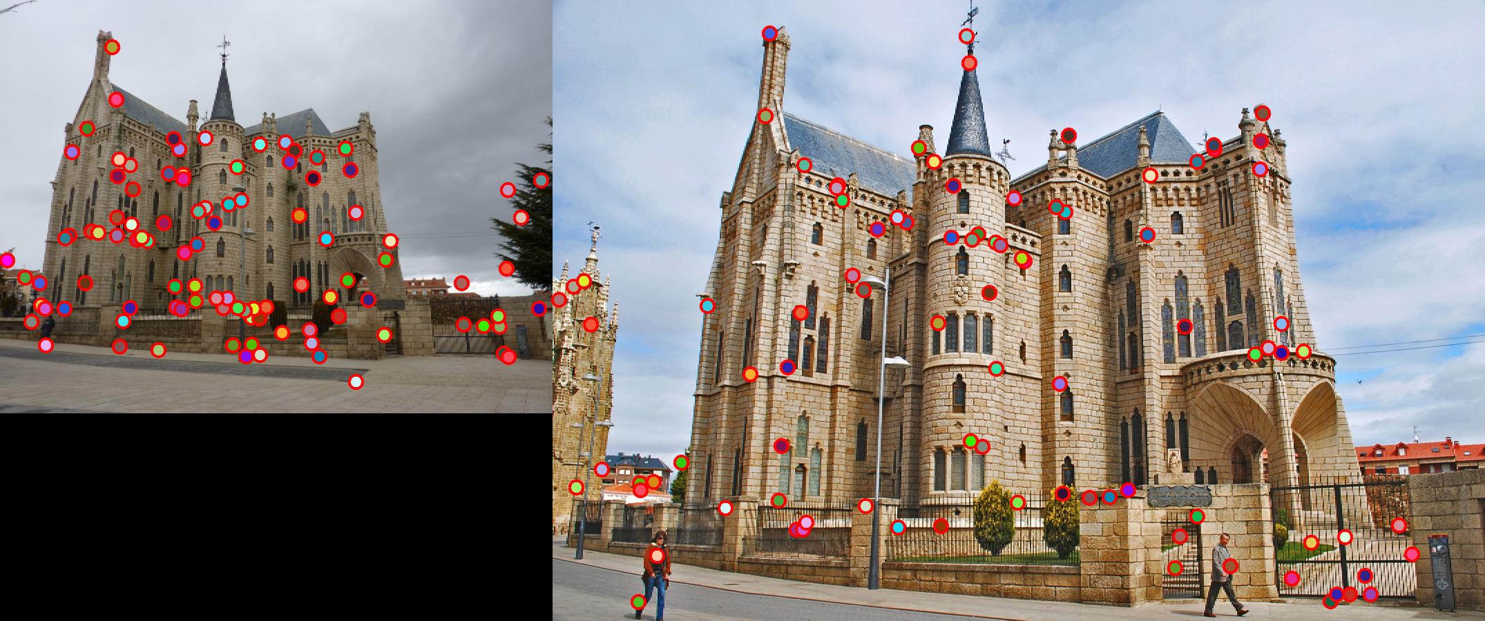
Episcopal Gaudi
The Episcopal Gaudi example consists of the following pairs of images,
The interest points obtained by our Harris detector are as follows,
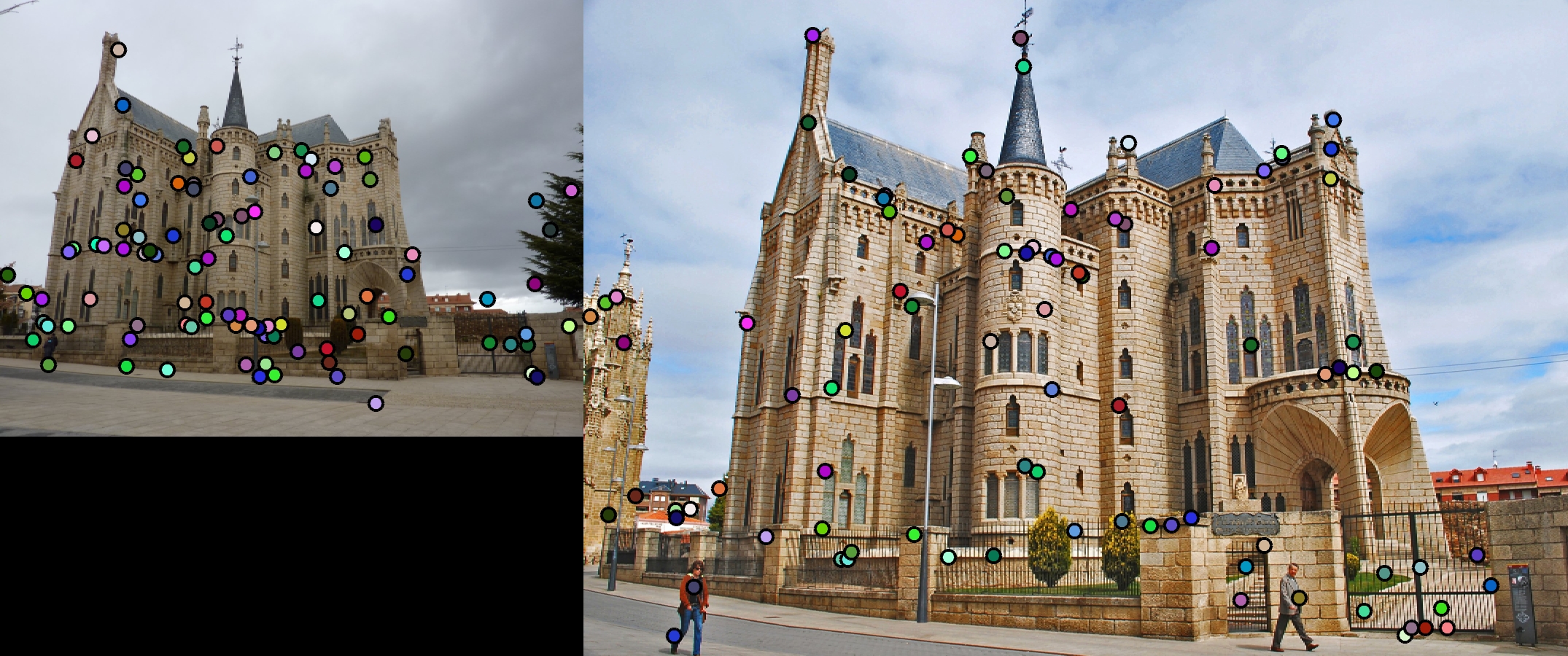
The interest points are obtained at points of sharp change in gradient and not on the smooth part of the image. Note that these are a sample of the interest points obtained by our detector and not the entire set.
Now we will look at the matches that our algorithm comes up with for the pair of images.
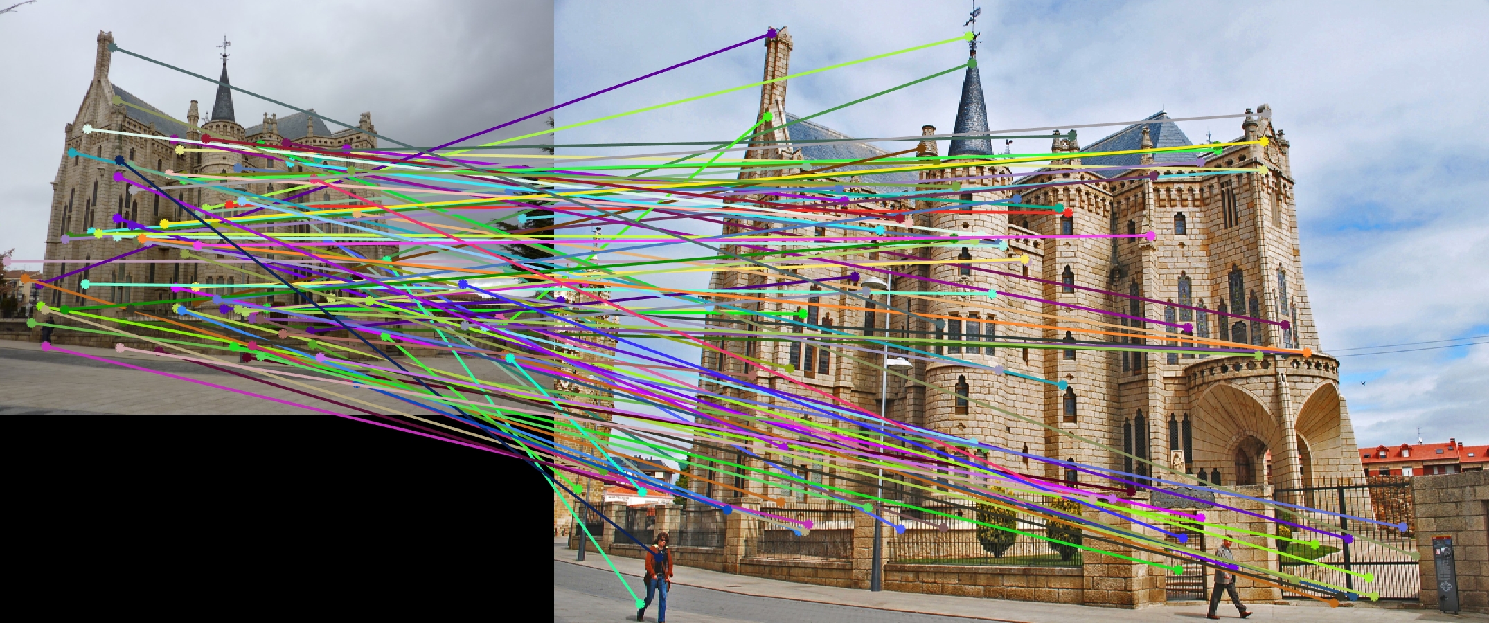
Most arrows go to points that are in the sameplace, though we do observe some strays. The strays represent places the algorithm has failed to build a good enough descriptor that can be deteccted later. The accuracy is 0%. The algorithm does not match any points. One reason for this can be the high difference in scale between the two points. The correct and incorrectly matched points are shown below.
Using PCA
We can use PCA to speed up matching by taking only the most relevant features that are required (aka dimensionality reduction). We use Matlab's in built PCA function to perform PCA. The number of features chosen is 32. In theory we should be able to speed up our matching by a factor of 4.
For forming universal bases, we need lots of data. In this case, we used the three pairs images as our data for calculating the universal bases. However, we can use more amounts of data to generalize our bases better.
When the non PCA implementation was run on the pairs of images, we got the following execution times for matching,
- Notre Dame - 0.983428s
- Mount Rushmore - 4.225537s
- Episcopal Gaudi - 1.102824s
- Notre Dame - 0.212564s
- Mount Rushmore - 0.899470s
- Episcopal Gaudi - 0.254877s
(We use the tic toc commands to find the time taken by matching)
Using KD Tree
We can use a KD Tree to speed up the matching of our features. This is beacuse the KDTree is optimized for nearest neighbour lookup. We used Matlab's KNNSearch implementation of a KD Tree to speed up matching. Since this was only optimizing the matching, it did not affect the accuracy of our algorithm. Matlab documentation mentions that the KDTree algorithm is more useful when the number of features is 10 or lesser, so we use our PCA implementation to take the 10 most important features.
When the non KD Tree implementation was run on the pairs of images, we got the following execution times for matching,
- Notre Dame - 0.112365s
- Mount Rushmore - 0.333537s
- Episcopal Gaudi - 0.092625s
- Notre Dame - 0.088596s
- Mount Rushmore - 0.198328s
- Episcopal Gaudi - 0.092557s
(We use the tic toc commands to find the time taken by matching)