Project 2: Local Feature Matching
Contents

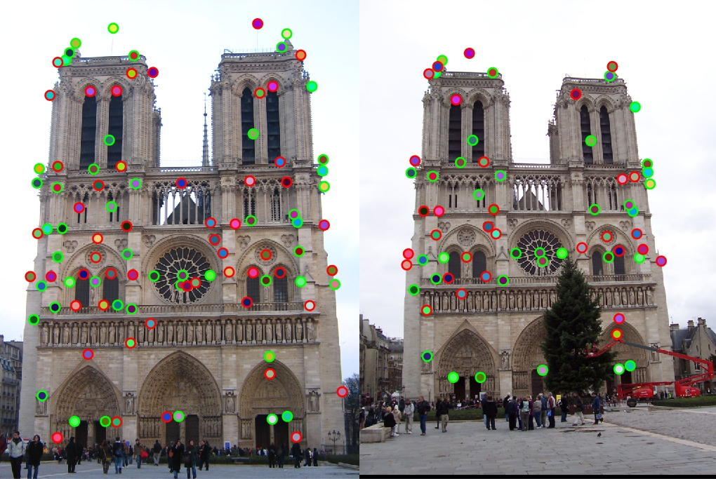
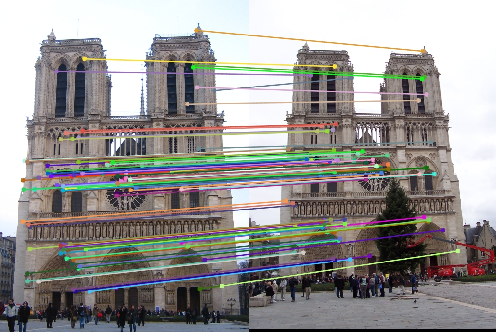
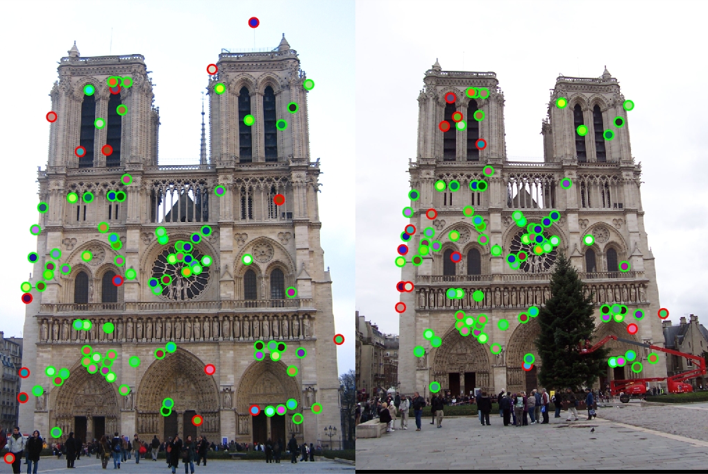
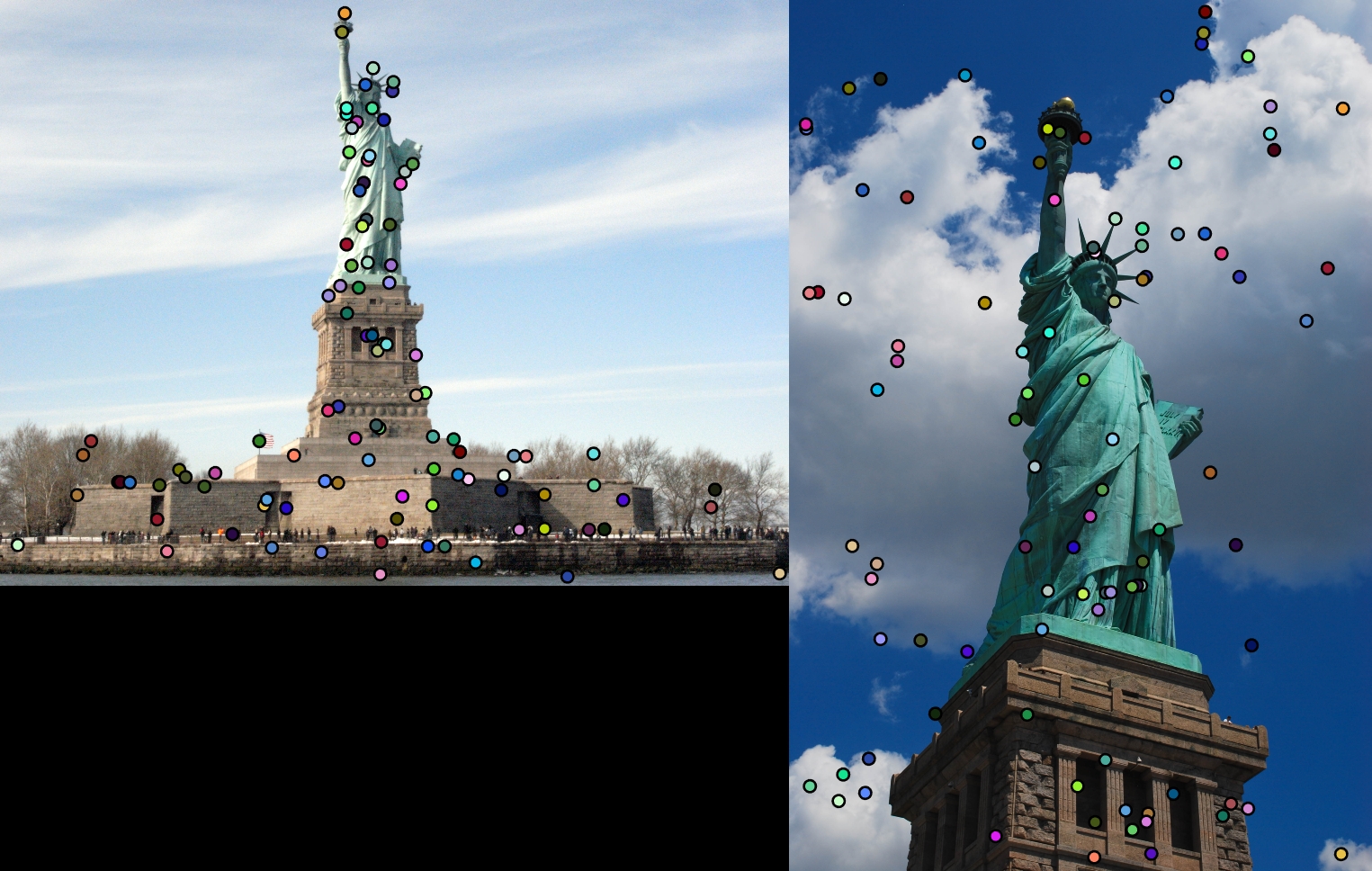
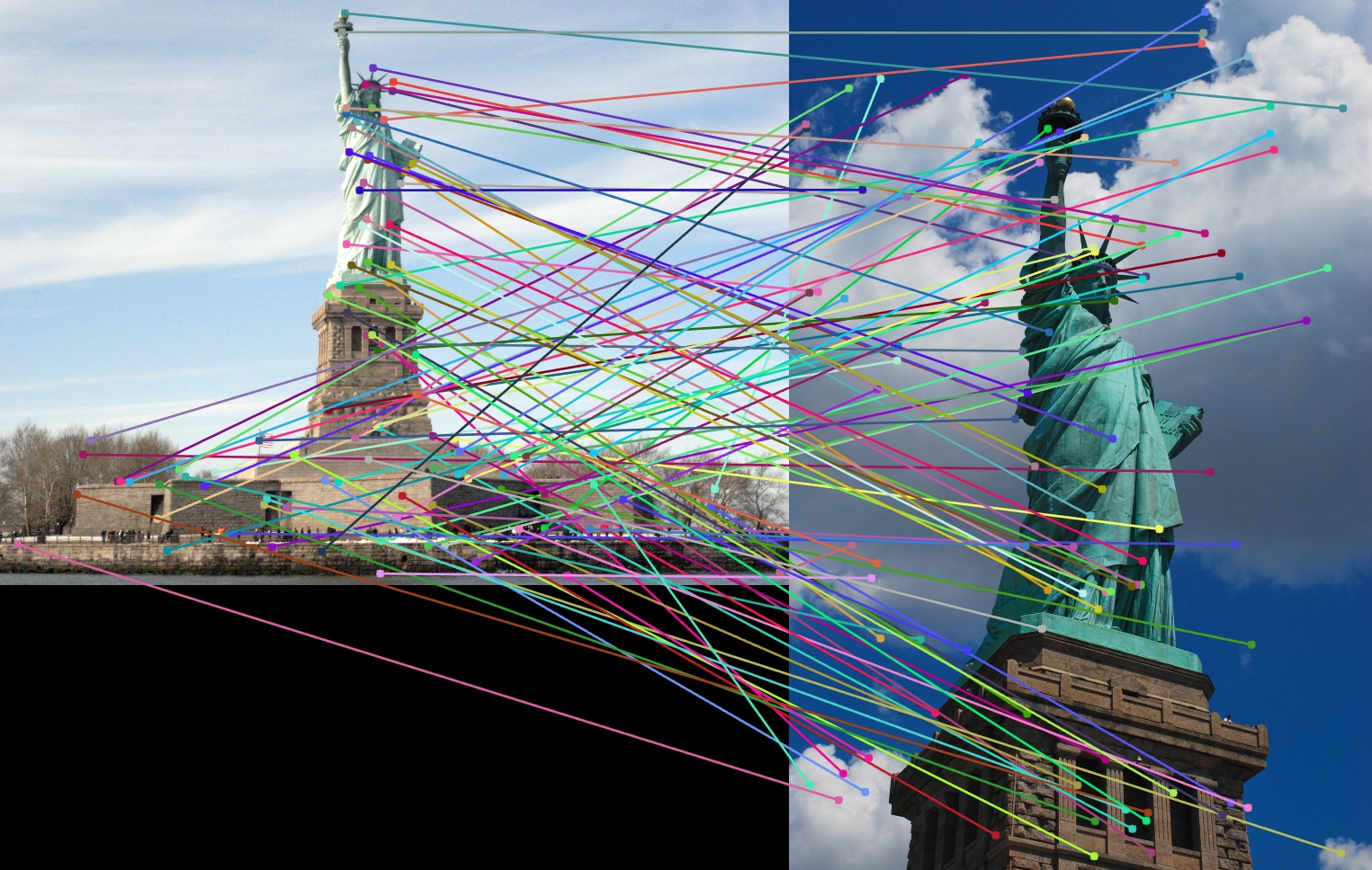
Example evaluation image
This project focused on the implementation of a local feature matching pipeline. The goal of the project was to implement the three major stages for a basic feature matching pipeline, including interest points with Harris Corners, feature descriptors with SIFT, and feature matching using the nearest neighbor method. This site discusses my results with implementing this pipeline as well as my reasoning for algorithm choices.
Algorithm Explanation
The basic feature matching pipeline can be split into three basic steps:
- Feature Matching
- SIFT Descriptor
- Harris Corners
The ordering of the pipeline for my discussion is actually in reverse order, as this was the order of implementation rather than the order of execution.
Feature Matching
The first step in my implementation was the completion of match_features.m, which uses the nearest neighbor algorithm in order to find the strongest potential matches between two sets of features. To do this, we first set up our necessary lists that will hold our matches and their confidence rating. Next, we want to loop through every feature from the first list, and compute the distance to every other point in the second list of features. We want to find the two nearest neighbors for each feature in order to calculate the correct confidence.
num_features = min(size(features1, 1), size(features2,1));
matches = zeros(num_features, 2);
confidences = zeros(num_features,1);
I decided to use pdist2, a built in matlab function, as it will compute the distance between a vector and every other vector in a provided matrix. This allows me to get a list of all of the distances from the current feature of interest to every feature in the second list. From this point, we can sort in ascending order so that the closest or nearest neighbors are in the front of the list. At this point, we can extract the distances for the two nearest neighbors, as well as the index for the nearest neighbor.
for i=1:1:size(features1, 1)

    dist = pdist2(features1(i,:), features2, 'euclidean');
    [dists, idxs] = sort(dist);
    nbors = dists(1:2);
    idx = idxs(1);
The next step is to calculate the nearest neighbor ratio by taking the nearest neighbor distance and dividing it by the second nearest neighbor distance. At this point, we could check for a threshold in order to eliminate bad matches, but this thresholding is implemented later by clipping to the 100 most confident matches or all matches if there are less than 100. Finally, we want to add the ratio to the list of confidences and the index of the features to the matches list. 1/ratio is added to the confidences rather than just the ratio in this case, because the sorting method used at the end is a descending sort. However, lower ratios are generally better, so doing 1/ratio will mean the smallest ratios will have the largest confidence and be sorted accordingly.
    ratio = nbors(1)/nbors(2);

    % 1/ratio so that lower (better) ratios have higher confidence
    % This also makes sure the descend sort has the best matches in front
    % rather than at the end so we can just take the 100 most confident
    confidences(i) = 1/ratio;
At this stage in the implementation, the correctness was still 0 since we were using random points of interest. The final code for feature matching can be seen below:
num_features = min(size(features1, 1), size(features2,1));
matches = zeros(num_features, 2);
confidences = zeros(num_features,1);

for i=1:1:size(features1, 1)
    dist = pdist2(features1(i,:), features2, 'euclidean');
    [dists, idxs] = sort(dist);
    nbors = dists(1:2);
    idx = idxs(1);

    ratio = nbors(1)/nbors(2);
    % 1/ratio so that lower (better) ratios have higher confidence
    % This also makes sure the descend sort has the best matches in front
    % rather than at the end so we can just take the 100 most confident
    confidences(i) = 1/ratio;
    matches(i,:) = [i, idx];
end

[confidences, ind] = sort(confidences, 'descend');
matches = matches(ind,:);
% Take the 100 most confident matches
if size(matches, 1) >= 100
    matches = matches(1:100,:);
Looping Over Channels and Padding
Next, since we are working with RGB images, we want to loop over all three channels and filter them separately. The code is written in a generic way to handle images of different numbers of channels as well. We simply extract the current channel from the image based on our index, and then use the built in MatLab function "padarray" to apply to correct amount of row and column padding to the image. The 'channel' variable is now our image we can apply the filter to.
% Create a pre-sized output array to hold final output
[img_rows, img_cols, channels] = size(image);
output = zeros(img_rows, img_cols, channels);

% Loop over the image channels
for i=1:1:channels
    % Get the current color channel and pad the array with 0's
    filt_channel = image(:,:,i);
    channel = padarray(filt_channel, [rowPad, colPad]);
SIFT-like Feature Descriptor
The next step in the implementation was to compute the feature descriptor for each of our keypoints of interest. I started by doing a very simple feature descriptor using the normalized patches from the image. Each of these patches was (feature_width x feature_width) and was simply the patch/norm(patch). The simple code for this is below:
for i=1:1:total_features

    col = round(x(i));
    row = round(y(i));
    % Get our 16x16 patch to process
    patch = image(row-pad:row+pad-1, col-pad:col+pad-1);

    features(i,:) = patch(:)/norm(patch);
end
Using this simple method, I was able to achieve 48% accuracy for the 100 most confident matches. At this point, I decided to apply a simple Gaussian blur to the entire image before processing the patches. This was to remove any erroneous features from the image that may have thrown off calculating. This ended up improving accuracy a surprising amount, coming in at 58% for the top 100 most confident matches.
Although this solution worked decently, we had to go ahead and implement a more SIFT-like feature descriptor. Overall algorithm for this was to extract our patches of the size of the feature width, computer the gradient magnitude for the patch, and then split this patch into 16 equally sized cells. After this, we bin the magnitudes into an 8 bin histogram for each cell based on the direction of the gradient.
To break this down in the code, we first filter with our Gaussian as stated earlier. Then, we loop through the features within the image to extract the x and y coordinate of our feature. We need to round these values since they are not integer values. Next, we simply extract our patch from the image, which is of size feature_width. Next, we want to compute the gradient within this patch to use for the descriptor. I decided to use imgradient, because it extracts both the gradient magnitude and direction for the patch. At this point, I add 180 to all values in the gradient direction matrix, which I will discuss the reason for later. Finally, I decided to use mat2cell to break the matrices into correctly sized blocks. I know this method may be slightly slower than just indexing into the matrix, but I like the simplicity of having actual split cells to work with in an array. The blocks are also split correctly based on our feature_width/4, which is the size of each cell.
total_features = size(x, 1);
features = zeros(total_features, 128);
pad = feature_width/2;

gauss_filt = fspecial('gaussian', [feature_width, feature_width], 1);
image = imfilter(image, gauss_filt);

% Our block size to use. Shortened to b_s for brevity in code
b_s = feature_width/4;
for i=1:1:total_features

    col = round(x(i));
    row = round(y(i));
    % Get our 16x16 patch to process
    patch = image(row-pad:row+pad-1, col-pad:col+pad-1);

    [gmag, gdir] = imgradient(patch);
    gdir = gdir + 180;
    % Weight the gradient magnitudes with our gaussian
    % I believe this was suggested in the algorithm, but it produced much worse results
    % gmag = gmag .* gauss;

    % Split our gradient magnitude and directions into 4x4 blocks
    mag_blocks = mat2cell(gmag, b_s*ones(1,4) , b_s*ones(1,4));
    dir_blocks = mat2cell(gdir, b_s*ones(1,4) , b_s*ones(1,4));
The next step in creating the SIFT descriptor is to process the individual cell blocks. I first initialize the 1x128 descriptor, and then begin a loop over the 16 cells from the image patch. I think create a 1x8 histogram vector that we will use in the binning process for each cell. This is where the addition of 180 degrees comes into play. The returned directions matrix from imgradient() has values in the range of [-180, 180]. The addition of 180 degrees puts these values in the range [0, 360]. For each of the 8 possible orientations, I calculate the 45 degree range that values must fall into, which starts with 0-44.9, and adds 45 for each orientation bin. I use some matlab operators to create a boolean matrix to find which values fit the current bin, and then take the total sum of all of those values from the magnitudes block. I can then store this summed value into the corresponding histogram bin for all 8 orientations. Once this is done for a cell block, I add it in the correct place within the current feature, and I finally add the new feature to the full list after normalizing it.
feature = zeros(1,128);
for j=1:1:4
    for k=1:1:4
        bins = zeros(1, 8);
        mags = mag_blocks{j,k};
        dirs = dir_blocks{j,k};
        for ori=0:1:7
            fits = ((dirs >= ori*45) & (dirs <= ori*45+45));
            total = sum(sum(mags(fits)));
            bins(1,ori+1) = total;
        end
        f_idx = (j-1)*32+(k-1)*8+1;
        feature(f_idx:f_idx+7) = bins;
    end
end
% normalize the feature and add it to the list
features(i,:) = feature(:)/norm(feature);
At this stage in the implementation, I was still using cheat_interest_points, and was able to achieve an accuracy of 65% for the Notre Dame set.
The final code for the SIFT-like descriptor is below:
total_features = size(x, 1);
features = zeros(total_features, 128);
pad = feature_width/2;
gauss_filt = fspecial('gaussian', [feature_width, feature_width], 1);
gauss = fspecial('gaussian', [feature_width, feature_width], 8);
image = imfilter(image, gauss_filt);

% Our block size to use. Shortened to b_s for brevity in code
b_s = feature_width/4;
for i=1:1:total_features

    col = round(x(i));
    row = round(y(i));
    % Get our 16x16 patch to process
    patch = image(row-pad:row+pad-1, col-pad:col+pad-1);

    [gmag, gdir] = imgradient(patch);
    gdir = gdir + 180;
    % Weight the gradient magnitudes with our gaussian
    % I believe this was suggested in the algorithm, but it produced much worse results
    %gmag = gmag .* gauss;

    % Split our gradient magnitude and directions into 4x4 blocks
    mag_blocks = mat2cell(gmag, b_s*ones(1,4) , b_s*ones(1,4));
    dir_blocks = mat2cell(gdir, b_s*ones(1,4) , b_s*ones(1,4));

    feature = zeros(1,128);
    for j=1:1:4
        for k=1:1:4
            bins = zeros(1, 8);
            mags = mag_blocks{j,k};
            dirs = dir_blocks{j,k};
            for ori=0:1:7
                fits = ((dirs >= ori*45) & (dirs <= ori*45+45));
                total = sum(sum(mags(fits)));
                bins(1,ori+1) = total;
            end
            f_idx = (j-1)*32+(k-1)*8+1;
            feature(f_idx:f_idx+7) = bins;
        end
    end
    % normalize the feature and add it to the list
    features(i,:) = feature(:)/norm(feature);
end
Harris Corner Detector
The final stage in my implementation was the addition of the Harris Corner detector algorithm to extract features from the image. The implementation of this method removed the need for cheat_interest_points, as it allows me to extract my own features from any image. The Harris Corner Detector algorithm has a couple of free parameters that I have found to affect the final accuracy quite significantly, which will be discussed in a later section. This section discusses the core elements of my Harris Corner Detector implementation
The first step in the algorithm is to apply a Gaussian blur to the entire image. This is to help eliminate some possible poor features such as a crack in a wall or something that like. It just slightly smooths the image so stronger corners remain. After this, I used imgradientxy() to extract the image gradient of the image in both the X and Y directions. These matrices are the base components for our Harris Corners algorithm
fw = feature_width;

% Good alpha value typically in range of 0.04 to 0.15 taken from
% http://www.cvc.uab.es/~asappa/publications/C__ICIAR_2013_LNCS_7950_pp_354_363.pdf
alpha = 0.04;
gauss = fspecial('Gaussian', [fw fw], 1);
% Blur before getting derivatives
image = imfilter(image, gauss);
% Get our derivatives
[Ix, Iy] = imgradientxy(image);
The next step in the process is to remove everything from the image near the edges of the image. We don't want to have interest points near the edge because it causes our SIFT-like feature to go out of bounds, or requires the use of padding, which could throw the descriptor values off if we used zero padding. This step just quickly lets us zero out these near-edge areas so they do not become interest points
% Get rid of everything near the edges so SIFT doesn't go out of bounds
% I imagine there is a more concise way to do this, but this at least
% removes the correct points from being used in harris calculation
Ix(1:fw,:) = 0;
Ix(end-fw:end,:) = 0;
Ix(:,1:fw) = 0;
Ix(:,end-fw:end) = 0;
Iy(1:fw,:) = 0;
Iy(end-fw:end,:) = 0;
Iy(:,1:fw) = 0;
Iy(:,end-fw:end) = 0;
The following step is to calculate our Harris Matrix elements that will be used to find the "cornerness" of points within the image. This is done by taking our earlier computed gradient images and multiplying them to get our Ix^2, Iy^2, and Ixy. We must then take each of these matrices and filter them with a Gaussian in order to get our final matrix elements. Finally, with these elements, we could either arrange them in a square matrix and used the determinant formula to calculate the cornerness at each pixel individually, or we can do it using matrix calculations, which I have done in my code. This computes a matrix of the same dimension as our image that we can then threshold and extract relevant interest points from.
% Compute our matrix elements
Ix_2 = Ix.*Ix;
Iy_2 = Iy.*Iy;
Ixy = Ix.*Iy;

% Filter the matrices with a separate gaussian
% In this case it's actually the same as the first Gaussian
% but I wanted to try different filter sizes and sigmas to see their effect
gauss2 = fspecial('Gaussian', [fw fw], 1);
GIx_2 = imfilter(Ix_2, gauss2);
GIy_2 = imfilter(Iy_2, gauss2);
GIxy = imfilter(Ixy, gauss2);

% Compute our final Harris matrix
harris = GIx_2.*GIy_2 - GIxy.*GIxy - alpha*(GIx_2+GIy_2).*(GIx_2+GIy_2);
The next and final steps of the Harris Corner Detector are to threshold our Harris matrix, perform non-maxima suppression, and extract the remaining strong interest points. I decided to first threshold the image by using the simple matlab expression to set any values less than the threshold to zero. The threshold parameter was a strong free parameter that was very important in achieving higher accuracy. It has a large tradeoff between number of interest points and the overall accuracy. The next step was to perform non-maxima suppression. This step was key in removing interest points within a window so that we don't have too many interest points right beside each other. Applying a very small window for this sliding window actually increased the accuracy greatly (managing to get up to 98%), but had the tradeoff of a drastically increased runtime as colfilt is an expensive operation. I also noticed that using a smaller window was more accurate because it found many features within smaller neighborhoods.
The last step in this process was to remove the suppressed values from the harris matrix using a similar technique as thresholding. In this case, I decided to check for values in the suppressed matrix to find the ones that matched the original values in the harris matrix. This meant that the value wasn't suppressed, so we wanted to keep those and set everything else to zero. We can then use a simple find() on the harris matrix to extract the coordinates of the strongest interest points, which we need to flip so that they can be correct x and y coordinates. We then add the corresponding confidence levels to our confidence matrix to finish the Harris corners.
threshold = mean2(harris);
% Threshold our Harris matrix to remove other points
harris(harris < threshold) = 0;
% Apply non-maxima suppresion using colfilt
% I noticed that for Notre Dame, applying a smaller filter size
% Improved the accuracy greatly from 84% to 92% for 100 most confident
% Applying an even stricter filter resulted in 97% accuracy, but greatly
% increased run time since the number of points goes up drastically
maxima_winsize = fw/2;
suppression = colfilt(harris, [maxima_winsize maxima_winsize], 'sliding', @max);
% Find where un-suppressed values exist and
% Remove all non-maxima from the harris matrix
harris(harris ~= suppression) = 0;
% Get the coordinates of our strongest features
[y, x] = find(harris > 0);
% Set our confidence value for the remaining features
confidence = harris(harris>0);
After the implementation of the Harris Corner Detector, accuracy increased up to 84% with the basic parameters. With different parameter tuning throughout the pipeline, I was able to achieve accuracies in the range of [84%, 98%] for Notre Dame, although the higher accuracy range certainly had a lot of clustered points. The final code without comments, as well as results can be seen below:
fw = feature_width;

alpha = 0.04;
gauss = fspecial('Gaussian', [fw fw], 1);
image = imfilter(image, gauss);
[Ix, Iy] = imgradientxy(image);

Ix(1:fw,:) = 0;
Ix(end-fw:end,:) = 0;
Ix(:,1:fw) = 0;
Ix(:,end-fw:end) = 0;
Iy(1:fw,:) = 0;
Iy(end-fw:end,:) = 0;
Iy(:,1:fw) = 0;
Iy(:,end-fw:end) = 0;

Ix_2 = Ix.*Ix;
Iy_2 = Iy.*Iy;
Ixy = Ix.*Iy;

gauss2 = fspecial('Gaussian', [fw fw], 1);
GIx_2 = imfilter(Ix_2, gauss2);
GIy_2 = imfilter(Iy_2, gauss2);
GIxy = imfilter(Ixy, gauss2);

harris = GIx_2.*GIy_2 - GIxy.*GIxy - alpha*(GIx_2+GIy_2).*(GIx_2+GIy_2);

threshold = mean2(harris);
harris(harris < threshold) = 0;
maxima_winsize = fw/2;
suppression = colfilt(harris, [maxima_winsize maxima_winsize], 'sliding', @max);
harris(harris ~= suppression) = 0;
[y, x] = find(harris > 0);
confidence = harris(harris>0);
More Results
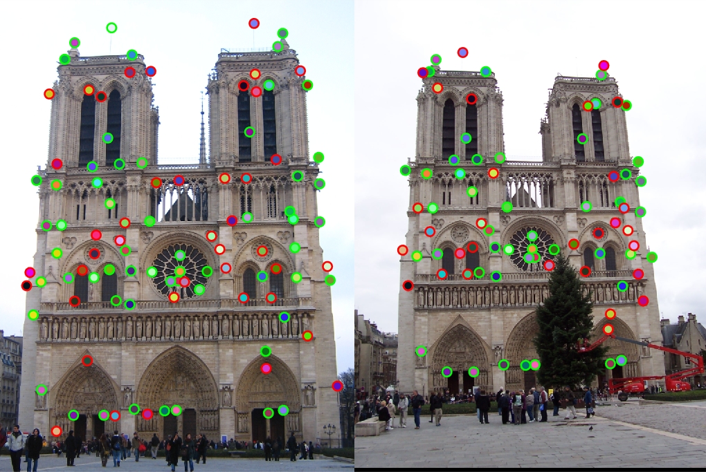
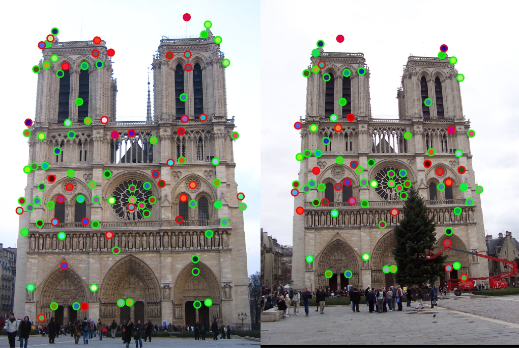
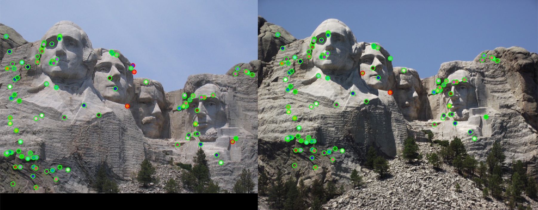
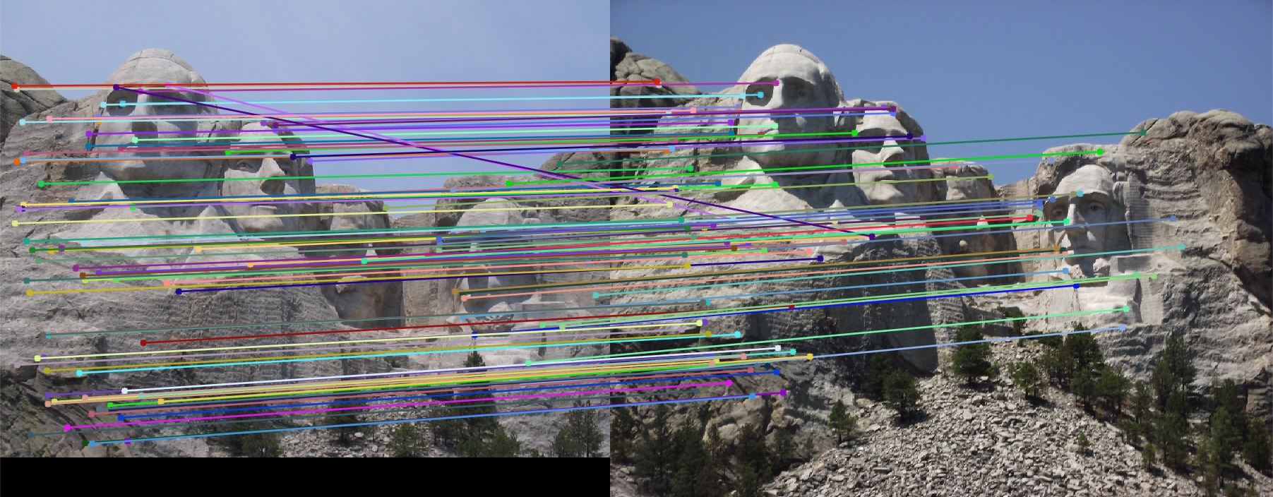
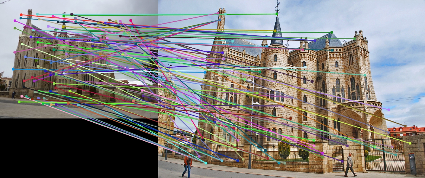
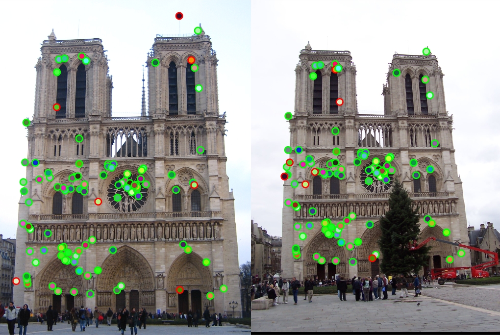
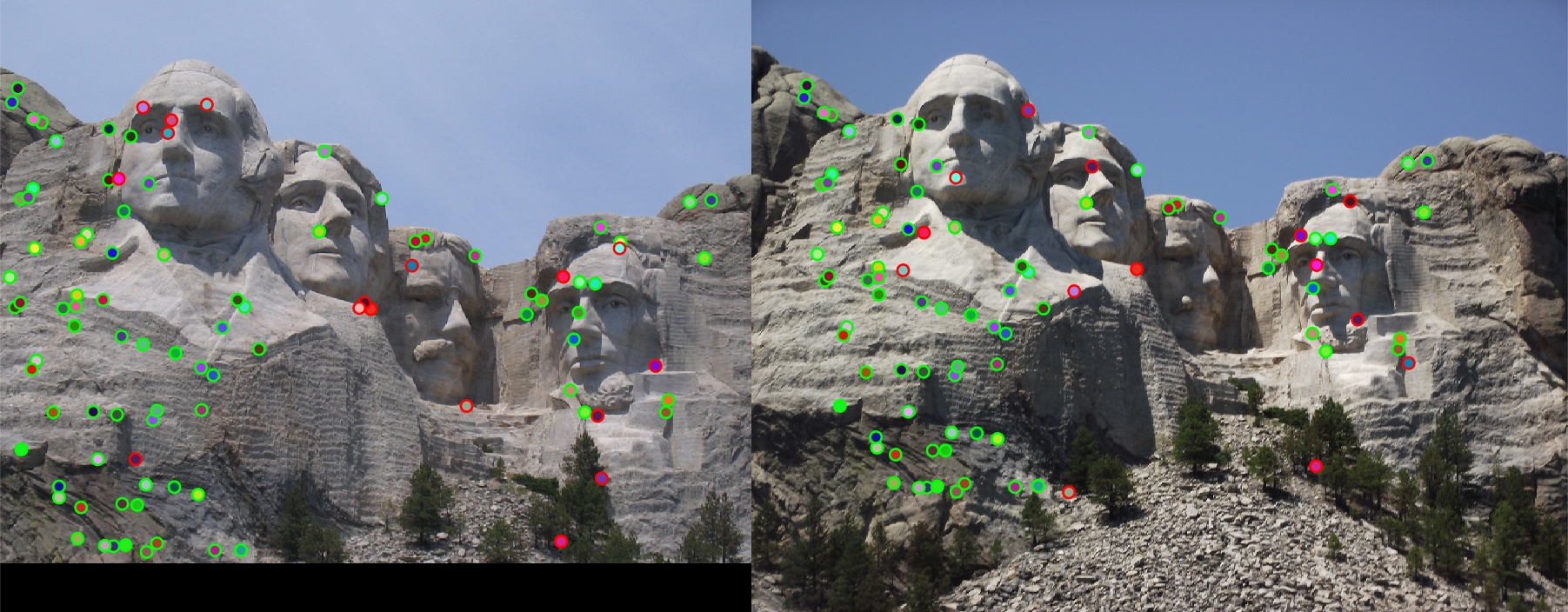
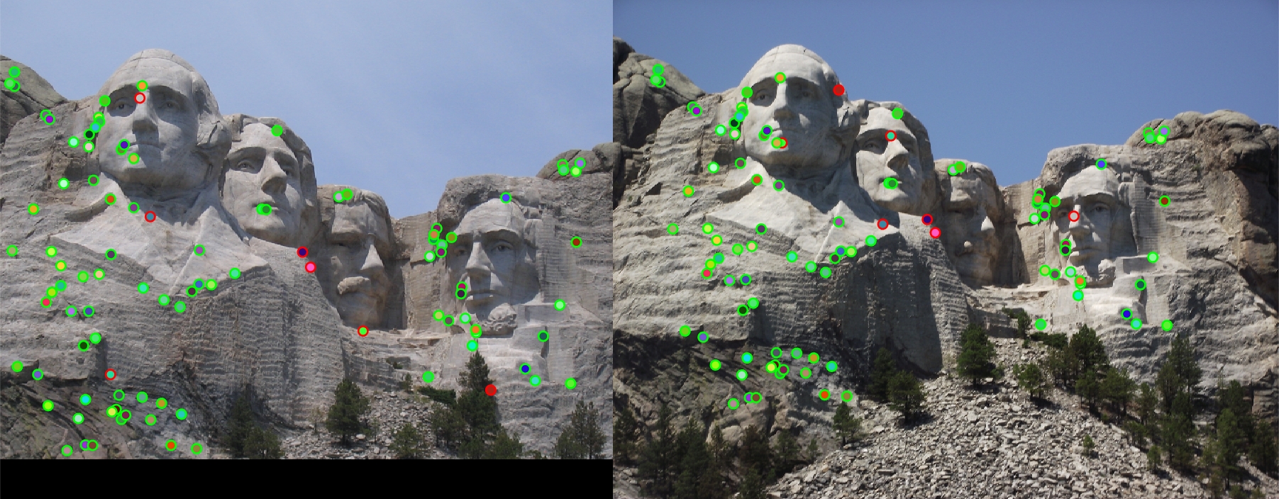
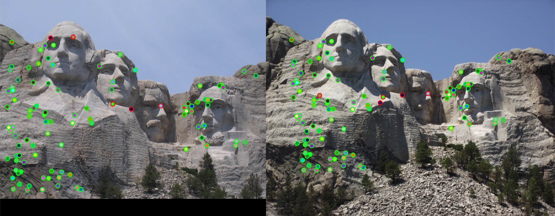
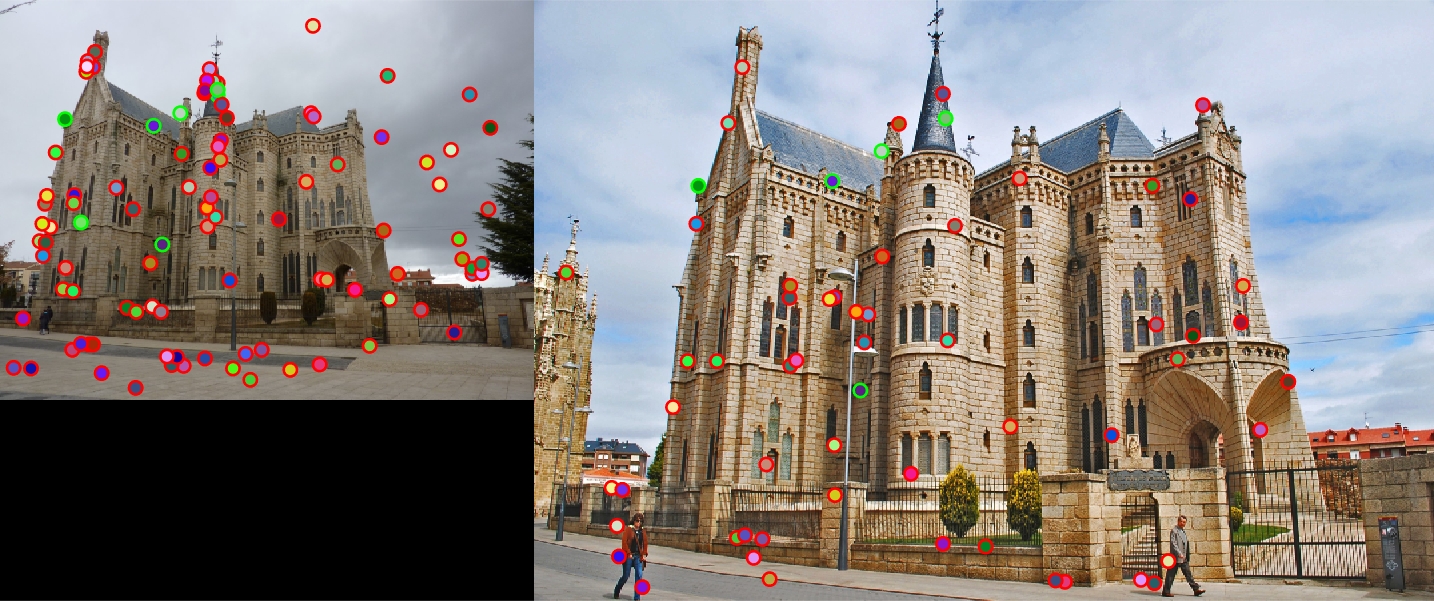
With lots of parameter tuning, which is discussed below, my final best results for matching accuracy can be seen below. I was able to do particularly well with Notre Dame and Rushmore, but for some reason my pipeline did not work well with Gaudi. I wasn't able to pinpoint the exact cause of this, which is why the results for that pair seem so bad. I also noticed that due to the smaller window size I used for maxima suppression, my best features were relatively clustered
|
|
|
|

|
|
Parameter Tuning
The full feature matching pipeline has a very large number of free parameters that can affect the accuracy of the overall matching. Some of these features include sigmas for Gaussians, the alpha and threshold values in the Harris Detector, the window size when performing non-maxima suppression, and the size of our feature width. This section discusses how some of these free parameters affected the match accuracy as well as the number of features found.
Gaussians
There are a very large amount of Gaussian filters present within the pipeline. I found that both the application and parameters of the Gaussians had either little or significant effect on the accuracy of the feature matching. For example, the first applied Gaussians in the Harris detector seemed to have the best effect with lower sigma values. I ended up settling on a sigma of 1 and window size equal to the feature_width. This Gaussian is applied to the entire image at the beginning as well as to each of the gradient matrices we compute. I tried applying separate Gaussians at this stage, but ended up getting the best results by using the same Gaussian to filter both.
Another important Gaussian was the first one applied before creating the SIFT-like descriptors for our features. Similar to the Harris Detector Gaussian, I found that a Gaussian with a window size equal to the feature_width as well as a sigma value of 1 produced the best results. Larger sigma values had a negative effect on accuracy while changes in window size had overall negligible effects. I also tried to apply a Gaussian filter to the gradient magnitude of the patch in order to try and suppress the effects of points farther from the interest points. I believe this was suggested as part of the pipeline, but I found that it negatively effected the accuracy of the final result
Alpha and Threshold
These parameters were key components of the Harris Corner Detector. Tuning of the alpha parameter was relatively easy. This parameter was used in the creation of the Harris Matrix, and after doing some research, I found that the generally accepted best values were in the range of [0.04, 0.15]. For my experimentation, I found that an alpha of 0.04 produced the best results in this case. The threshold was a little bit trickier. I noticed that using a threshold of 0 was generally good, and gave me a percentage of 84% with no other tuned parameters. This was consistent with every other threshold I tried, even the larger range of -1 or 1 as a threshold. After some more research on this parameter as well, I settled on using the mean value of the harris matrix as my threshold, as this generally gave good results.
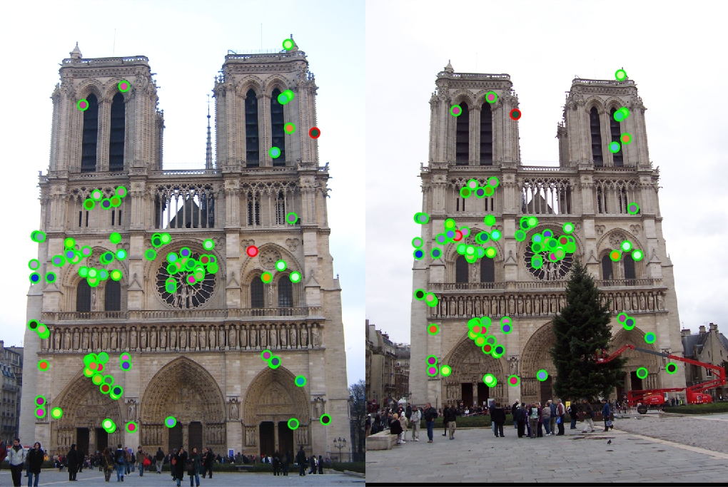
Non-Maxima Suppression Window Size
This was a parameter in the pipeline that seemed to have a very strong effect on the final accuracy of the results. At first, I used a window size in the colfilt function equal to the feature width. Overall, this produced fairly good results. For the Notre Dame pair, I achieved 84% accuracy and 83% accuracy for the Rushmore pair. By simply decreasing the size of my maxima suppression filter in the colfilt, I was able to achieve 93% for Notre Dame and Rushmore. The noticeable difference was in the runtime. By cutting the feature window in half, I was essentially causing the function to run 4 times as many filters. This greatly slowed down the execution time. I even experimented with a window size of feature_width/4, which gave me up to 97% accuracy with tuned parameters for Notre Dame, but the execution time was extremely long in comparison to the smaller window sizes. Making this feature smaller also drastically increased the number of interest points by thousands, which wasn't very desirable.
|
|
|
|
|
|
Feature Width
I also found that changing the feature_width parameter had some good effects on my final results. For example, with some parameters tuned, feature width of 24 instead of 16 increased the accuracy on Rushmore from 83% to 95%, which is a very drastic change. Also, on Gaudi, I was able to slightly increase, achieving accuracies of 7% and 11% for feature widths of 16 and 64 respectively.
|
|
|
|
|
Further Results
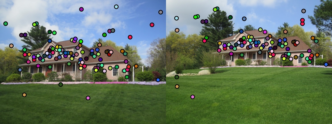
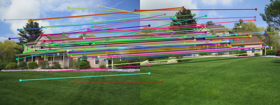
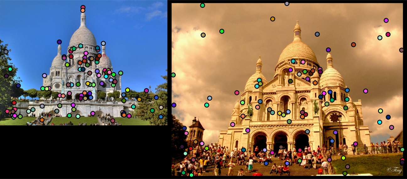
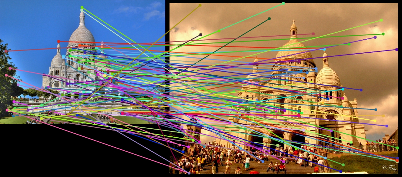
I also attempted to use some of the extra image pairs. The house seemed to match quite well, but this is probably due to similar alighment and illumination. The other pairs did not fair as well.
|
|
|
|
|
|