Raj Prateek Kosaraju

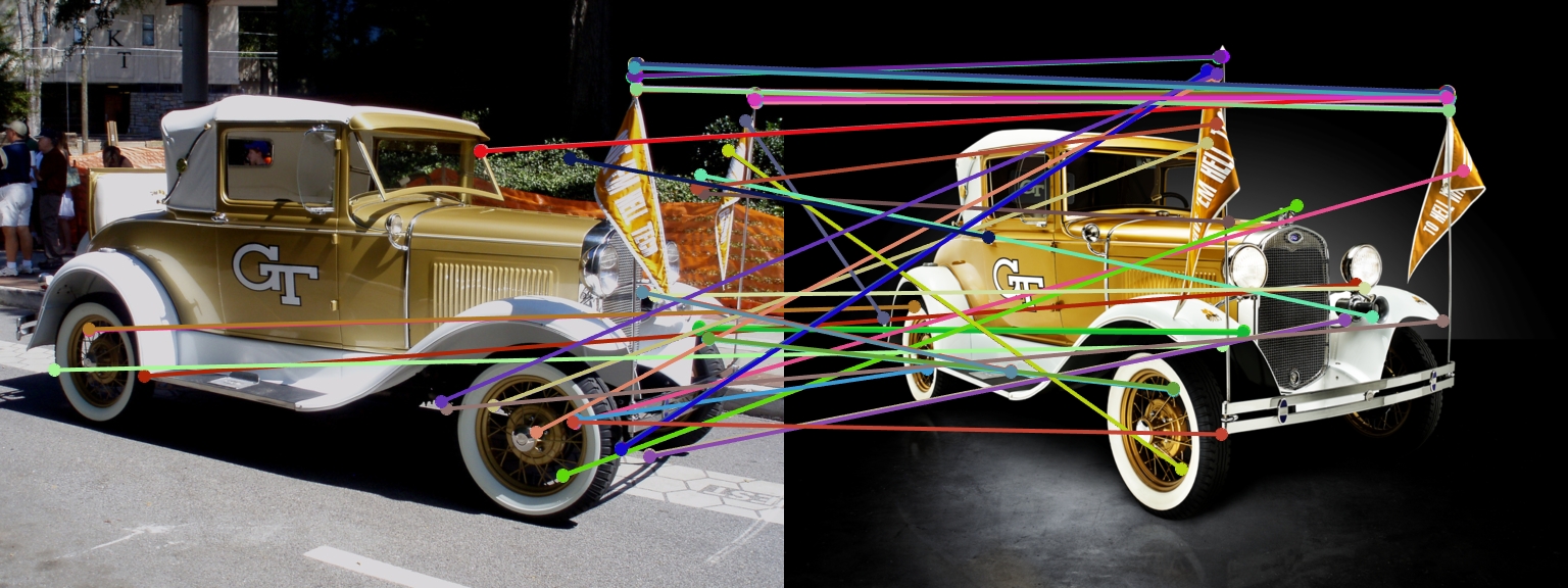
A matched image of the Ramblin Wreck. The lines indicate matched features.

Interest Point Detection

The first and foremost step such a task would be to detech points in each of the image that are of interest. These points would be the ones that the algorithm would build off of in the next few steps. The detector essentially tries to pick points that are distictive in nature- distiguishable from their surrounding pixels. Harris corner detector is a detector that can be used to achieve this task.

Applying the detector

I first compute the image gradient (using a sobel filter as it seemed to work better than gaussian), and then Ix^2, Iy^2 and Ixy. I plug these terms into the harris score equation and filter using a threshold. I also tried supression but it didn't seem to improve results in any of the cases. I also vary adjust the threshold (initialized to 0.3) and scale (initialized to 1) of the image dynamically, depending on if too few or too many interest points are detected.

%Code for the main part of the detector
gaussianFilter = fspecial('gaussian',feature_width.^2,2);
Ix = imfilter(image,fspecial('sobel'));
Iy = imfilter(image,(fspecial('sobel')));
Ixx = imfilter(Ix.*Ix,gaussianFilter);
Iyy = imfilter(Iy.*Iy,gaussianFilter);
Ixy = imfilter(Ix.*Iy,gaussianFilter);
harris = (Ixx.*Iyy - Ixy.^2) - alpha*(Ixx + Iyy).^2;
harris(harris < threshold) = 0;
[y,x] = find(harris);

Local Feature Description

This step involves using a vector to describe each of the points that we detected from the previous step. This is essential to be able to compare points in the future and to be able to accurately match the corresponding points. I first started with normalized patches as suggested but this gave bad results. Notre dame was giving an accuracy of low 60s%. I then implemented a SIFT like feature description by following Lowe's paper. This immediately improved the accuracy to the 85% to 92% range.

SIFT steps

To implement the SIFT-like feature descriptor, I computed the x and y graident of the image, and the magnitude and orientation of the gradient. Then, for each of the points of interest, we split it up into 4*4 cells and bin the angles into 8 bins. We then keep appending this to the features ofn the point until we finish for all 16 cells, leaving us with a 128 dimension feature for each point. After computing this for all such points, we also normalize the feature matrix.

Feature Matching

This step involves taking the points of interest and vectors describing them for two differenting and macthing corresponding points of interest. To do this, we perform a nearest neighbor ratio test as described in Szeliski 4.1.3

Finding the matches

We first compute the distance between each interest point's feature from image1 to each interest point's feature from image2, giving us a matrix of distances. We then compute the ratio by dividing the closest neighbor for each point with it's second closes neighbor. This also acts as a measure of inverse confidence as if this value was high, then the second closes neighbor may also be a good candidate and we aren't sure which one would be a good match.

Below is a code snippet that illustrates how this is done in matlab.

%matching code
threshold = 1- 0.9275;
distances = pdist2(features1, features2);
[asc_distances, mapping] = sort(distances, 2);
nndr = (asc_distances(:,1)./asc_distances(:,2));
confidences = 1- nndr;
thresholded_confidences = confidences(confidences>threshold);
matches = zeros(size(thresholded_confidences,1), 2);
%get x matches
matches(:,1) = find(confidences>threshold);
%get y matches
matches(:,2) = mapping(confidences > threshold, 1);
confidences = thresholded_confidences;
% Sort the matches so that the most confident onces are at the top of the
% list. You should probably not delete this, so that the evaluation
% functions can be run on the top matches easily.
[confidences, ind] = sort(confidences, 'descend');
matches = matches(ind,:);

Bells and Whistles

During interest point detection, the code tries to dynamically update the scale of the image and the treshold it uses to find interest points if there are too few points being identified. The resulting interest points are also adjusted to be with respect to the original scale of the image and the correct scale matrix is returned. I also experimented with the SIFT parameters to see if any changes could consistently give good results. I experimented with it to have both 9 bins and 7 bins instead of 8. 9 bins gave a slightly worse accuracy than 8 (low 70s for Notre Dam) while 7 bins seemed to have reduced the accuracy altogether to 44%. Changing the number of cells (making it 5*5 instead of 4*4) did not result in an increase in accuracy either. However, I did not try changing the number of cells and changing the number of bins at the same time.

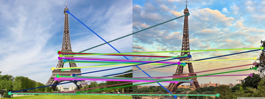
Results: Matched Images

Below are some of my results. The code has been modified to only calculate the accuracy using the 100 most confident matches.

Good results. 85 total good matches, 15 total bad matches. 85% accuracy Accuracy was also in the 91% at one point by varying thresholds.

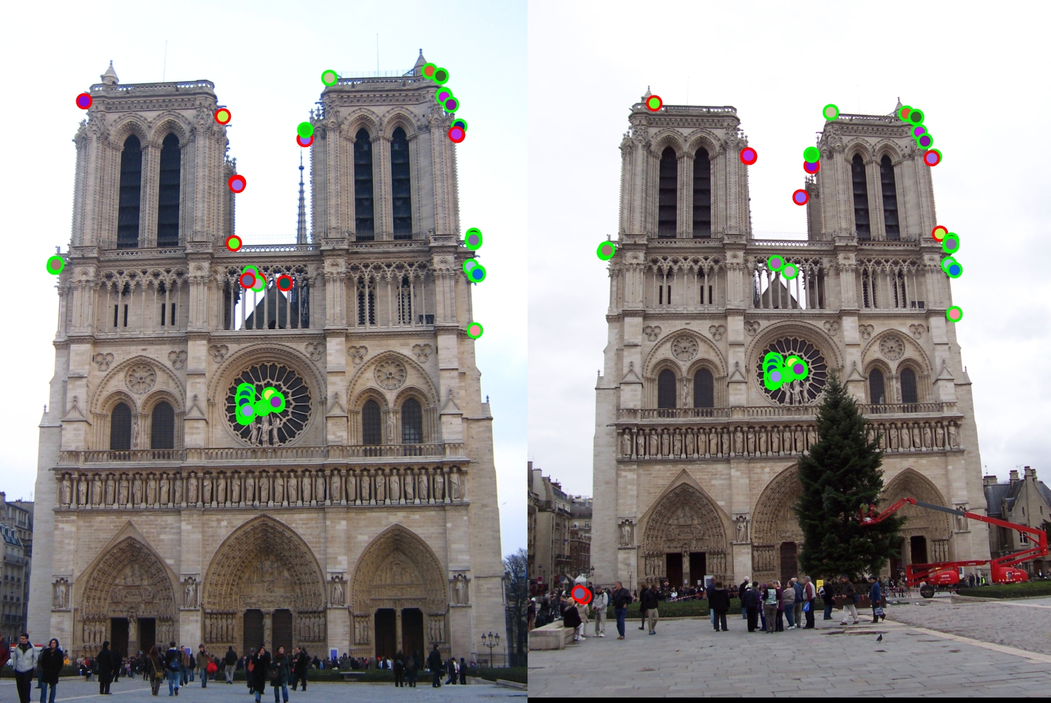
71 total good matches, 29 total bad matches. 71% accuracy

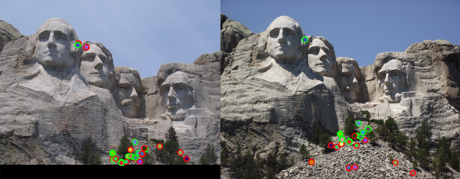
Bad results. Accuracy was in 7- 20% range regardless of minor threshold variations. I suspect this is due to the huge change in scale, which can't be anticipated until the feature matching step kicked in.

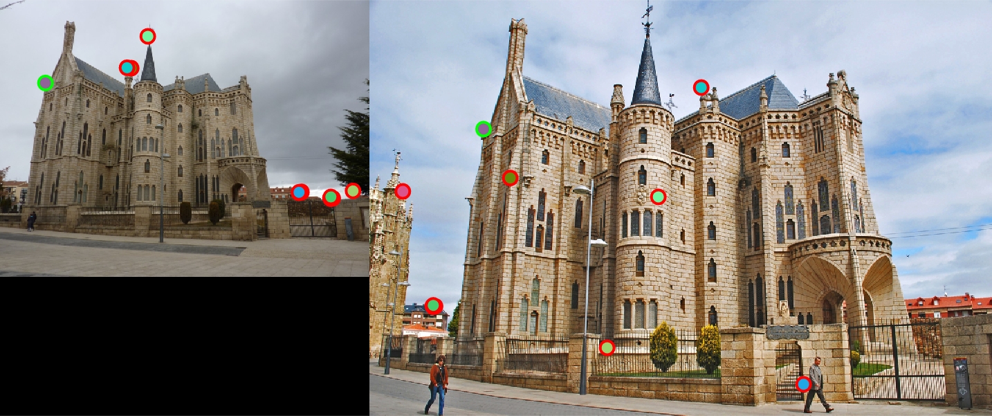
Good results! Seems like most of then important features got matched correctly.

Great results. Important features were identified and mostly matched well.