Project 2: Local Feature Matching
In this project, we were to create a local feature matching algorithm using simplified verseions of the SIFT pipeline. There were three main components of this project that we had to complete in order to match the features from two images correctly:
- get_interest_poinst.m
- get_features.m
- match_features.m
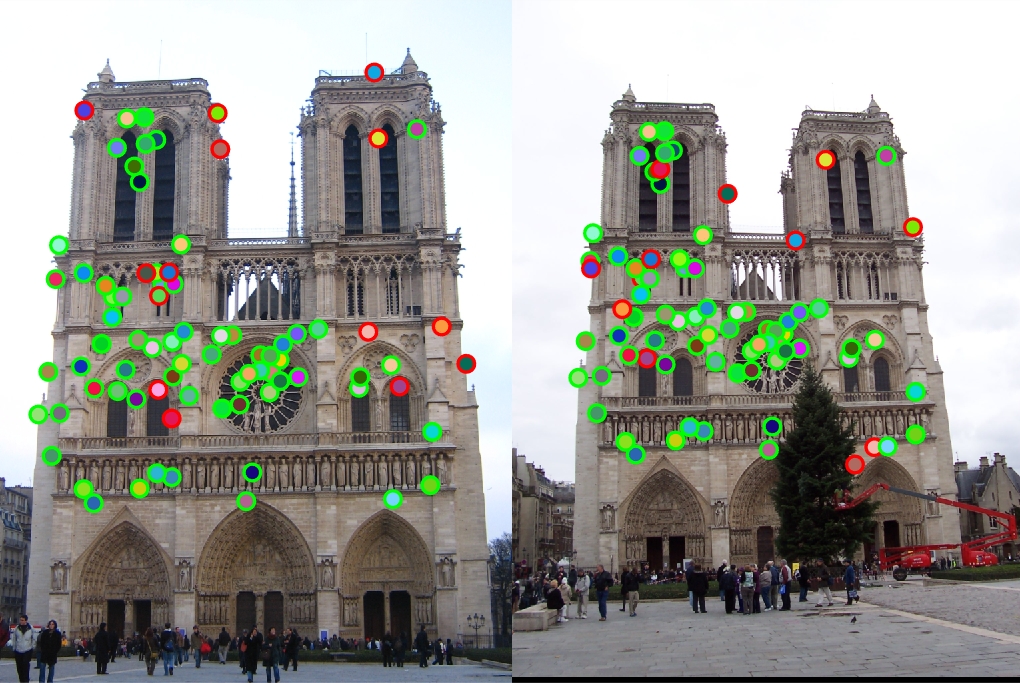
Interest Point Detection
In order to do interest point detection, I first computed the horizontal and vertical gradients of a gaussian when it was filtered with the image by taking the image derivatives. I then took the square of those derivatives and passed it through another gaussian filter. Using the cornerness function, I get the interest points.
% example code
% Getting the gradient of the image along the x and y axis
gaussian_filter = fspecial('gaussian', [15 15], 1);
[x_gradient, y_gradient] = imgradientxy(gaussian_filter);
Ix = imfilter(image, x_gradient);
Iy = imfilter(image, y_gradient);

% Finiding interest points
har = (g_Ix2 .* g_Iy2) - (g_Ix_Iy .* g_Ix_Iy) - alpha*((g_Ix2 + g_Iy2) .* (g_Ix2 + g_Iy2));
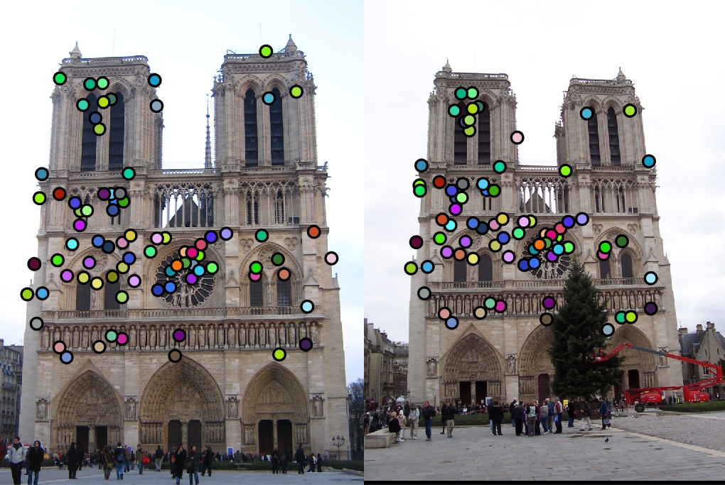
Get Features
For this method, I cut out image patches in order to get features. At first this didn't work because the image patches were going out of bounds, but I added some edge detection in order to only get the correct range of values for patches.
for i = 1:size(x)
    single_feature = zeros(1, 128);
    x_interest = x(i, 1);
    y_interest = y(i, 1);
    x_min = x_interest - (feature_width / 2 + 1);
    x_max = x_interest + (feature_width / 2);
    y_min = y_interest - (feature_width / 2);
    y_max = y_interest + (feature_width / 2 + 1);
    if x_min > 0 && x_max <= rows && y_min > 0 && y_max <= cols
        interest_area_mag = mag(y_min:y_max, x_min:x_max);
        interest_area_direction = direction(y_min:y_max, x_min:x_max);
        for j = 0:3
            for k = 0:3
                cell_size = feature_width / 4;
                cell_direction = interest_area_direction(j * cell_size + 1:(j+1)*cell_size, k*cell_size + 1:(k+1)*cell_size);
                cell_mag = interest_area_mag(j * cell_size + 1:(j+1)*cell_size, k*cell_size + 1:(k+1)*cell_size);
                for orient = 1:8
                    cell = sum(cell_mag(cell_direction == orient));
                    single_feature(1, 8 * (j * 4 + k) + orient) = cell;
                end

            end
        end

    end
    features(i, :) = single_feature / norm(single_feature);
end
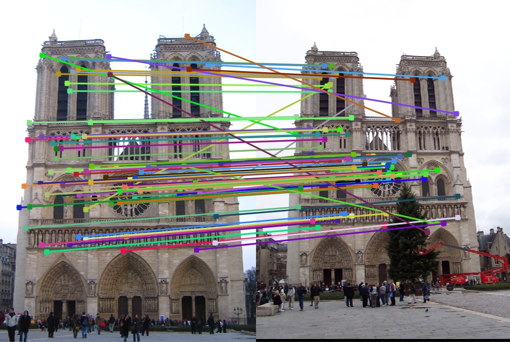
Match Features
In order to do match features, I found the ratio of the two closest features from one image to each feature in the other image. I used pdist2 to get the eucldiean distances, sorted the matrix that it returned, and used that to find the ratios from the first and second closest features.
threshold = 0.7;
feature_distances = pdist2(features1, features2, 'euclidean');
[distances_sorted, feature_indices] = sort(feature_distances, 2);
reverse_confidence = distances_sorted(:,1)./distances_sorted(:,2);
confidences = 1./reverse_confidence(reverse_confidence < threshold);

matches = zeros(size(confidences, 1), 2);
matches(:, 1) = find(reverse_confidence < threshold);
matches(:, 2) = feature_indices(reverse_confidence < threshold, 1);
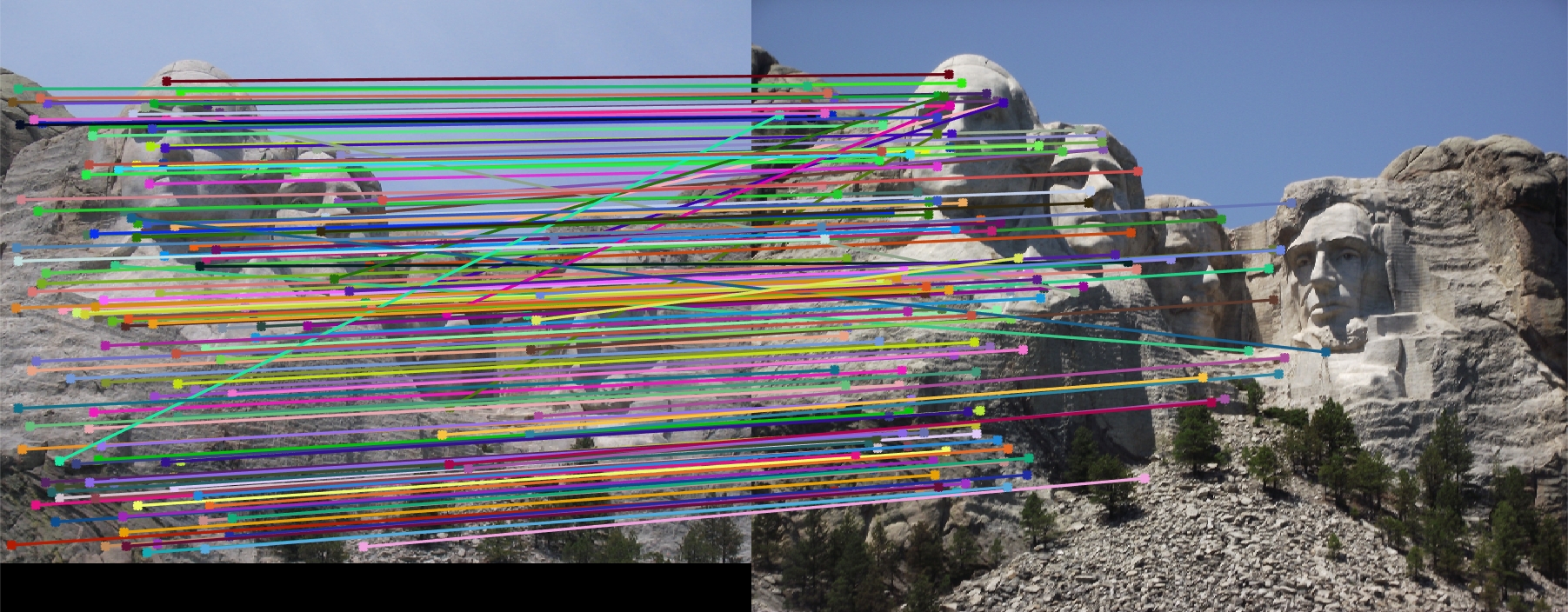
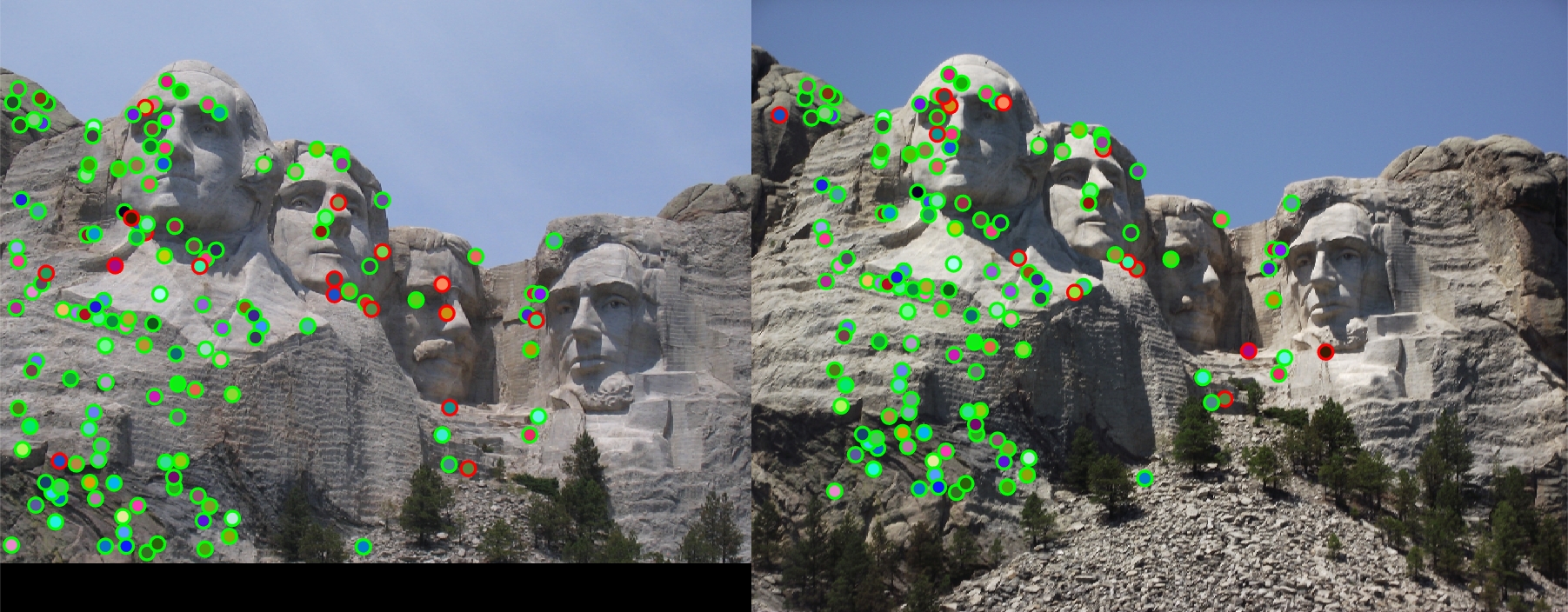
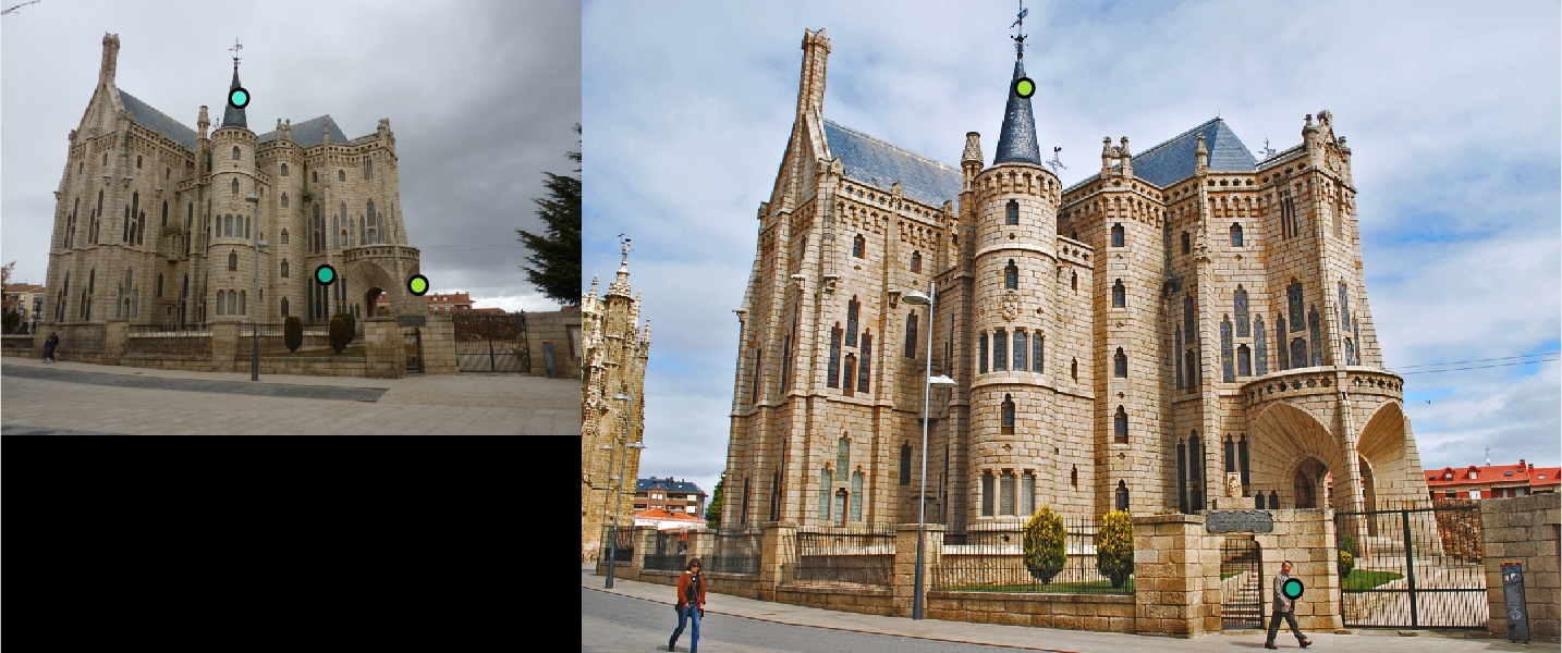
Results in a table
|
|


|
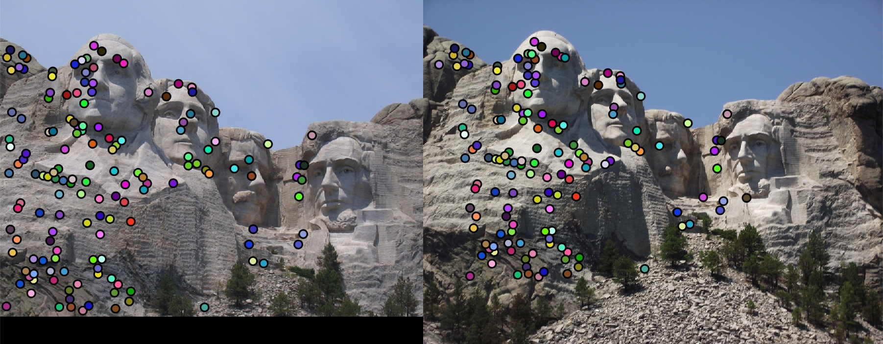
For the first set of pictures, the Norte Dame picture got an accuracy of 83% in terms of finding local features when compared with the ground truth correspondence. The Mount Rushmore pictures got an even better accuracy at around 89% accuracy. For some reason, the Episcopal Gaudi performed very poorly and stayed at 0%.