Project 2: Local Feature Matching
In this project, we implement local feature matching through the following steps:
- Generate interest points given an input image with the Harris corner detector.
- Create features at each interest point with the SIFT feature descriptor.
- Match the features to one another based on distance using the nearest neighbor ratio test to threshold out matches.
Generating Interest Points: Harris Detector
Interest points are created by computing the horizontal and vertical derivatives of the image. The image is blurred before this to produce better results. A cornerness function is used and the image is thresholded so that only points with a large corner response are returned. To furthermore reduce the interest points, only local maxima of those points are returned, which I tried with two methods 1) bwconncomp and getting the point in the component with the highest score 2) using a sliding window to compute local maxima. The first method did better than the sliding window--I think this is because the connected components method discarded a lot more of the weaker interest points than the sliding window method. Then, the x and y coordinates of the point, include the value output by the cornerness function (aka the confidence of the point) are returned.
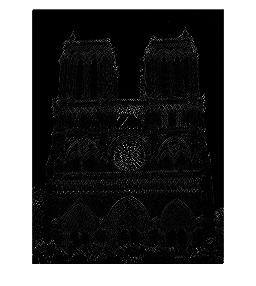
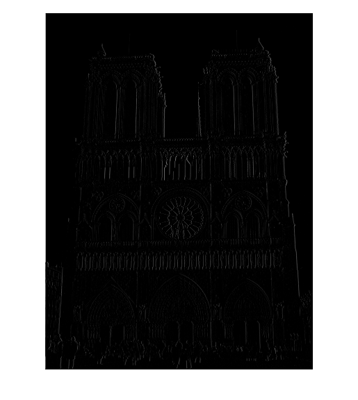
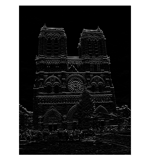
I experimented with the possible ways of taking the horizontal and vertical derivatives of the image, trying to compute the derivative myself, trying the derivative of gaussian suggested in the textbook, and finally, the derivative of Laplacian, which worked the best. You can try the possible ways in my code, I have Laplacian used, but that function can easily be changed to work with Gaussian, and I also have the horizontal/vertical derivative implemented (and commented out). The results of this can be seen below. Furthermore, you can see the difference between the interest points I discovered vs. the interest points that the Matlab implementation of the Harris detector discovered.
Discarding the interest points at the border of the image also helped, contributing to a 2% improvement in accuracy.

|


|
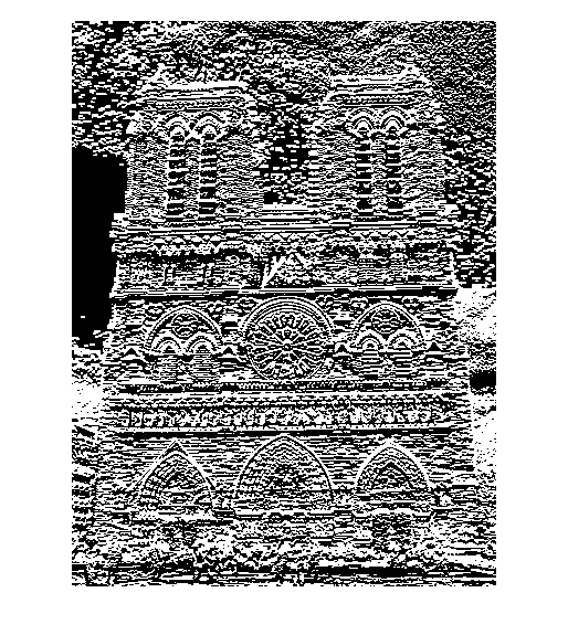
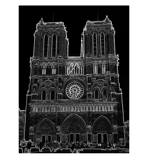
Left: filtering with derivative in x and y directions, Middle: filtering with derivative of gaussian, Right: filtering with derivative of Laplacian.
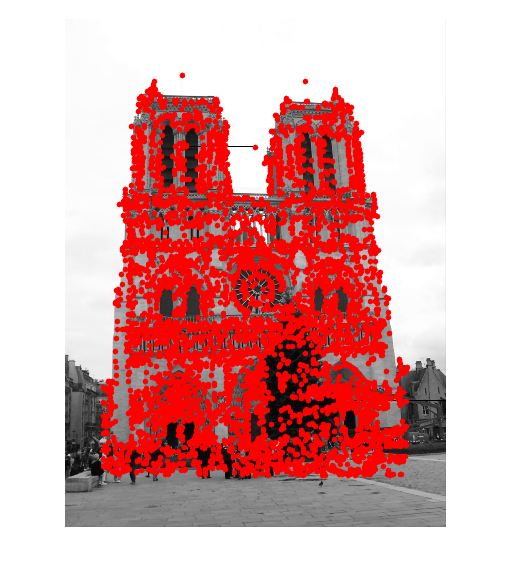
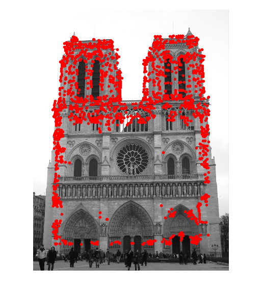
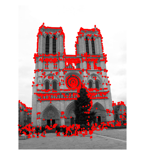
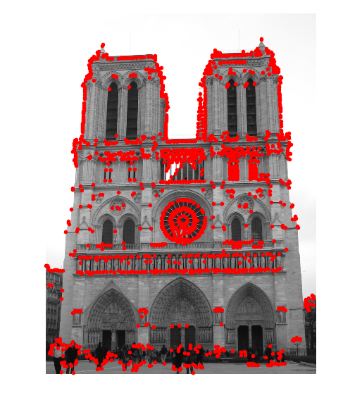
Left: interest points detected from my implementation of Harris, Middle, implementation of adaptive non-maximal suppression to 2750 points, Right: interest points detected from the Matlab implementation of Harris.
As you can see, I generate a lot more interest points than the Matlab implementation of Harris. While I could also decrease the number of interest points produced by changing the threshold value, it turns out that the number of interest points I produce dramatically affects my accuracy.With respect to the accuracy and different number of interest points generated, the theshold value for the cornerness function mattered--with each degree of magnitude, the percentage changed quite a bit.
| Threshold | Interest Points: Image 1 | Interest Points: Image 2 | Accuracy |
|---|---|---|---|
| .000008 | 7797 | 6655 | 79% |
| .00008 | 6972 | 5667 | 83% |
| .0008 | 6510 | 5355 | 82% |
| .008 | 2988 | 2926 | 77% |
| Gaussian Size | Gaussian Sigma | Accuracy |
|---|---|---|
| 5 | .1 | 79% |
| 5 | .3 | 84% |
| 5 | .4 | 91% |
| 5 | .5 | 0% |
| Threshold: # Interest Points | Accuracy |
|---|---|
| 4750 | 86% |
| 3750 | 79% |
| 2750 | 61% |
| 1750 | 43% |
| 750 | 19% |
Generating Feature Vectors
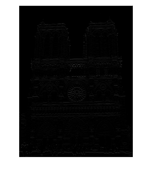
From the interest points, we can then compute feature vectors. This is done by taking a 16 x 16 pixel section around the interest point which then gets divided into a 4x4 grid of cells. For each cell, we compute a histogram based on the orientation of cell's gradient. The values added to the histogram are the magnitudes of the orientation. When it's just added like this, I achieve an accuracy of 89%. After adding some weighted binning of the magnitudes, I'm able to achieve 91% accuracy. With the weighted binning, I weight the two neighboring bins, if they exist, with .18 * the magnitude being added to the current bin. Finally, this results in a 1x128 feature vector per interest point and results in an nx128 list of features being returned. Features were normalized before being returned to between 0 and 1 by setting features = [ features - min(features) ] / (max(features) - min(features)). The other methods of normalization resulted in lower accuracies. One method I tried was features = features./norm(features), which resulted in 83% accuracy. The other method, L1 norm, features = features/sqrt(norm(features)^2+.01), resulted in 83% too. These two methods both performed worse than the first method, with an accuracy of 91%.
|
Left: orientation direction, Right: orientation magnitude.
Matching Features Across Images
Then, we match the features produced for each image. We first compute the distances between every pair of features. Then, we take the two closest features to a current feature and compute the nearest neighbor distance ratio--the ratio of the distance between the closest feature and our current feature divided by the distance between the second closest feature and our current feature. We can further threshold on this NNDR value, aka the confidence of our match, and throw out any matches that have low confidence. This results in a mx1 vector of confidences and a mx2 matrix of feature matches being returned. However, in my implementation, I chose to simply take the 100 highest confidences and their respective matches instead since it would pretty much do the same thing, except I was thresholding the number of matches returned rather than the confidence value.
My initial implementation involved simply computing the distances between every set of possible feature matches. From that matrix of distances, I would sort each row to retrieve the two lowest distances for the NNDR test. As part of the extra credit, I also used the Matlab implementation of k-nn, which allowed me to bypass computing the huge matrix of distances and instead use a k-d tree to return the 2 nearest neighbors to an input feature to compute the NNDR. The differences between the two matching implementations can be found in match_features.m (the original naive implementation) and match_features_extracredit.m (the k-nn implementation). While there's no difference between the two methods of implementation, the k-nn method was distinctly faster because computing the distances between every set of possible feature matches, especially when I had over 1000 features, was extremely time consuming.
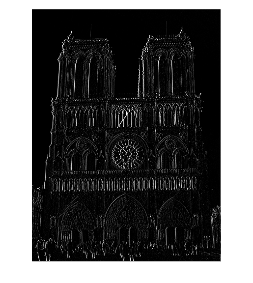
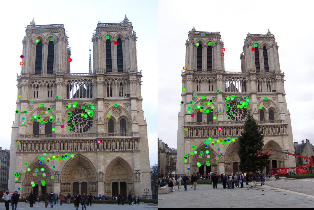
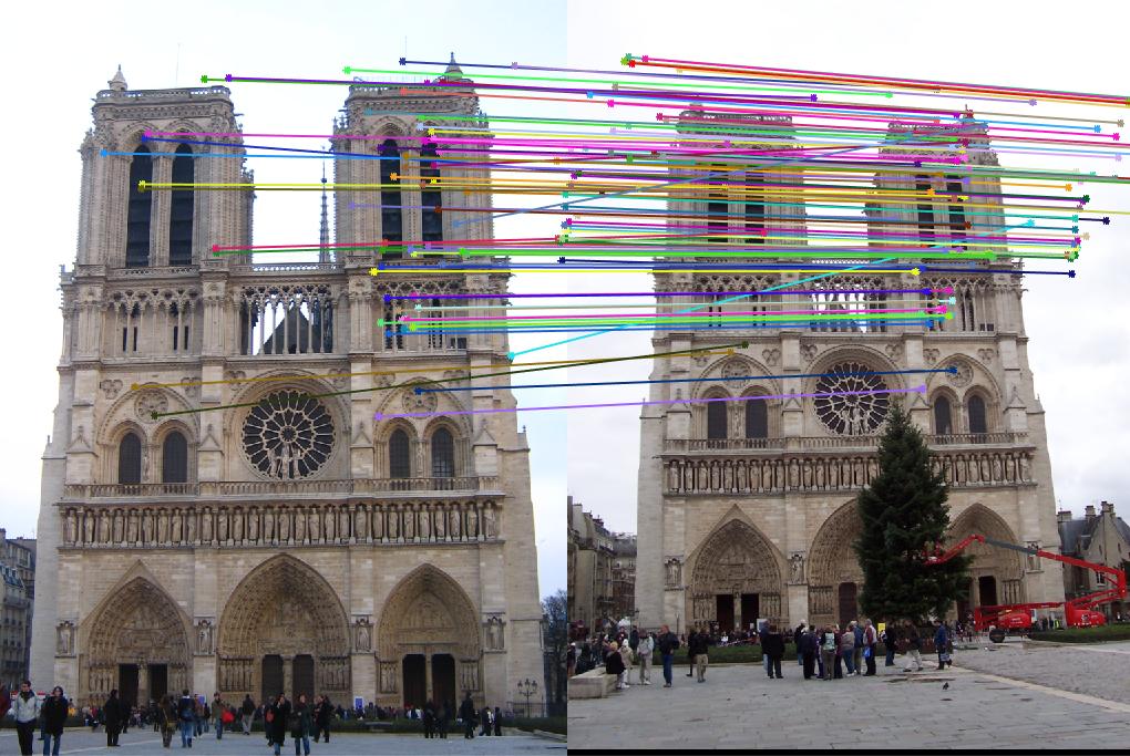
This results in an accuracy of 91% on the Notre Dame data, as shown below:
Results of Interest Points, Features, and Matches
|