Sidney Durant

Part 1: Interest Point Detection:

The technique used to find interest points in the original image is called the Harris corner detector. The Harris corner detector looks for distinctiveness (sometimes called cornerness) by local auto-correlation using a second moment matrix. High distinctiveness is needed for an interest point so that the exact location can be found. For example, finding points along an edge isn't helpful because any point along that edge may look similar. This is why finding corners (and looking to maximize cornerness) is so important. The Harris corner detector returns a list of interest points that can then be described by the local feature descriptors, and matched through feature matching.

There are several parameters to tune for the harris corner detector. One parameter that I did tune is the standard deviation of the gaussian used to blur the image before/after finding the gradients. Because the images weren't very noisy, I found that using a small standard deviation lead to the best results. (I used a standard deviation of 3 before calculating gradients, and of 1 after calculating the gradients.)

Part 2: Local Feature Description:

The next part of the project was to describe the features found in part one. To do this I used a SIFT like feature descriptor. This feature descriptor takes a 16x16 pixel image patch around each feature and proceeds to create gradient orientation histograms for each of the 16 4x4 cells within this image patch. The gradient orientation histograms are then normalized and put together. Because the gradient orientation histograms contain 8 bins, this creates a 1x128 (4*4*8) feature describing vector, which can then be used for feature matching. There were not many parameters to modify for this section. Using a SIFT like feature was much better than using image patches, as it raised accuracy from ~40% to 85% on the Notre Dame image pair.

Part 3: Feature Matching:

Part 3 of the project was to take the feature descriptions for each of the features and to try to find close matches between them. The output of this piece of code is a list of corresponding image points. (Of course the results aren't perfect, but for certain image pairs I was able to reach 85% accuracy. The results are discussed in detail later.) Feature matching is fairly straightforward. The algorithm starts by finding nearest neighbors among the 128 dimensional feature vectors. Then the algorithm finds the nearest neighbor distance ratio which is defined as the ratio between the nearest neighbor and the second nearest neighbor. This gives us a confidence rating of sorts. If a feature in image 1 seems to be very similar to a feature in image 2, then it will likely be a match, unless there are many very similar features. This is where the nearest neighbor distance ratio comes in: it's looking for pairs of features that have two properties: similarity to each other and dissimilarity to all other features. Points with a good nearest neighbor distance ratio are likely to be corresponding features.

Results:

I tested the code on three different image pairs. The first being the Notre Dame pair, the second the Mount Rushmore pair, and the last one being the Episcopal Gaudi pair. The code did well on the Notre Dame pair because the two images were taken from very similar viewpoints and with very similar illumination. Performance went down for the Mount Rushmore pair (where illumination is inconsistent) and then plummeted on the Episcopal Gaudi pair (where both illumination and scale are very different). The results of the full pipeline are shown in the table below. Note that for each image pair I show the results using both my interest point finder and ground truth correspondance. This makes it easier to see what part of the pipeline is failing for each of these image pairs.

Image Pair	# Good Matches	# Bad Matches	Accuracy
Notre Dame	90	16	85%
Notre Dame Cheat	102	58	64%
Mount Rushmore	6	12	33%
Mount Rushmore Cheat	38	48	44%
Episcopal Gaudi	0	14	0
Episcopal Gaudi Cheat	6	72	8%

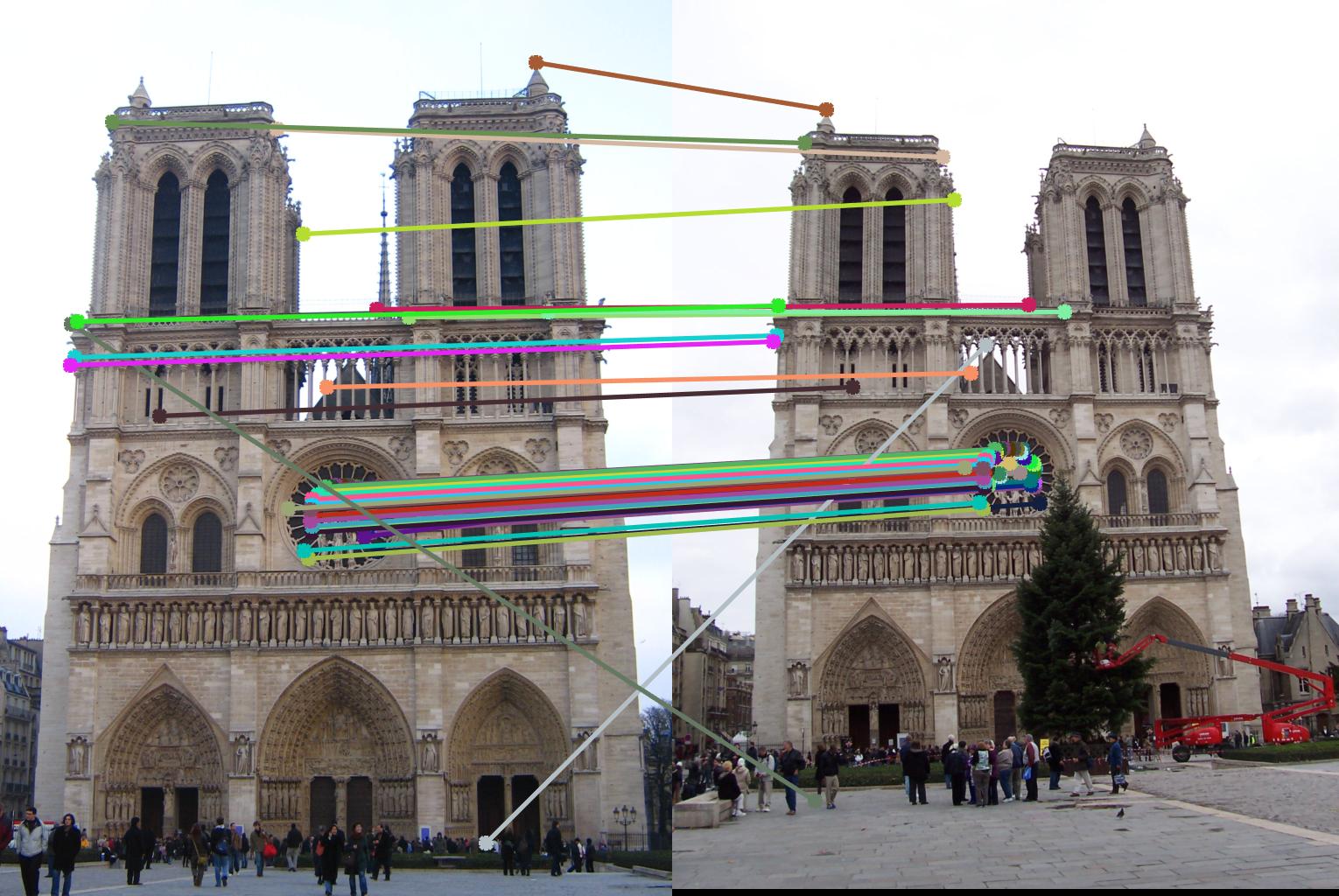
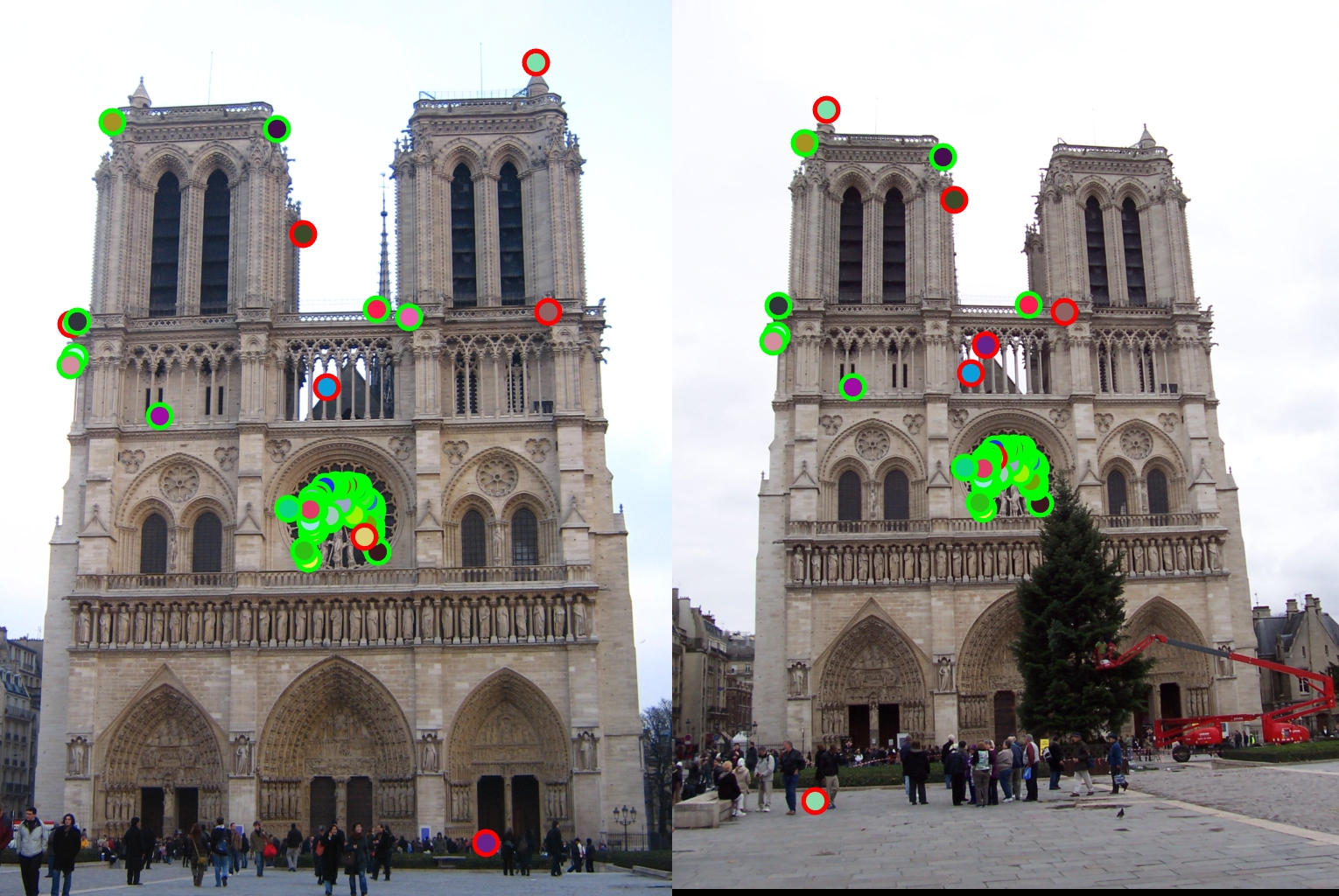
Notre Dame:

The pipeline performed well for the Notre Dame image pair. There were 90 good matches and 16 bad matches for this image pair; in other words there was 85% accuracy. It seems that the code had no trouble finding interest points, and that both feature description and feature matching worked well here. Using the ground truth correspondance interest points actually led to worse results than using generated interest points. This is likely because there are many many generated interest points, and so it is easy to find at least a few points that have a very high matching confidence (nearest neighbor distance ratio).

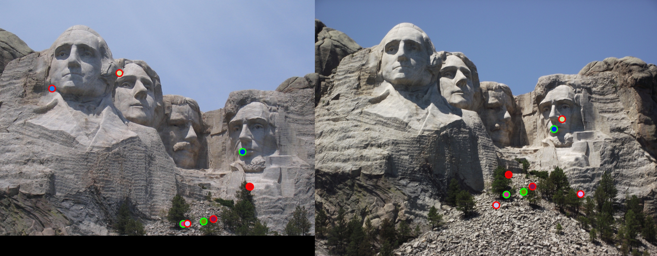
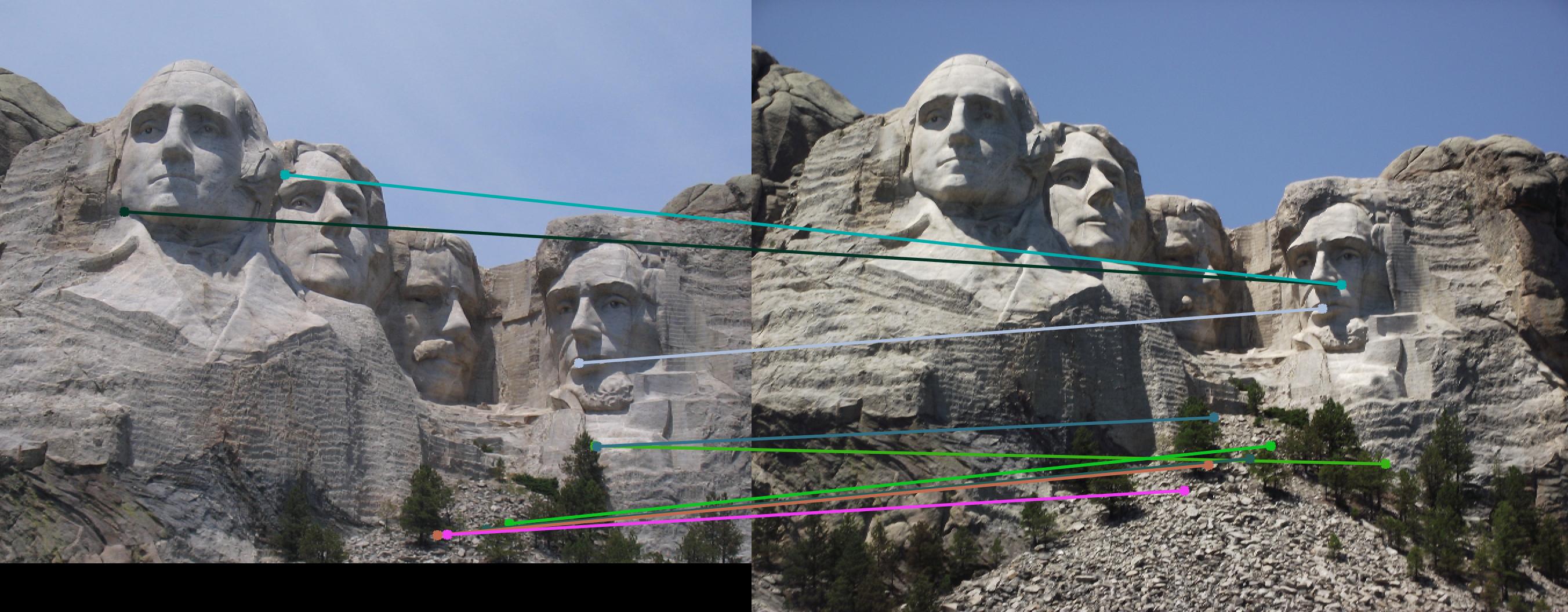
Mount Rushmore:

The pipeline did not perform as well on the mount rushmore image pair. For the full pipeline, there was 33% accuracy. Using the existing ground truth interest points, there was 44% accuracy. There seems to be trouble with finding the same interest points in both the left and right image (likely due to different illumination) so although the second half of the pipeline works well, the interest points found are different for both the left and right images and so they cannot be successfully matched. Using cheat interest points still leads to reasonable results (using Hough transform it is likely that one could figure out which points are correct and get rid of the other (incorrect) matches).

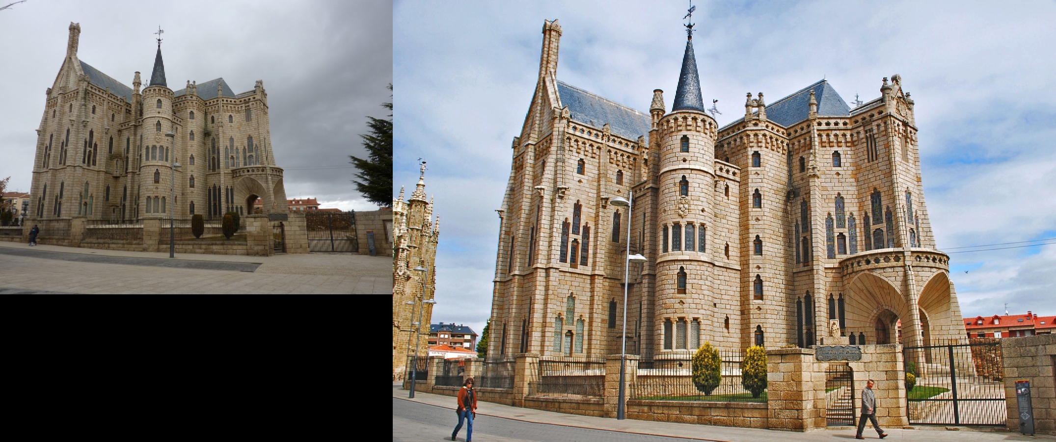
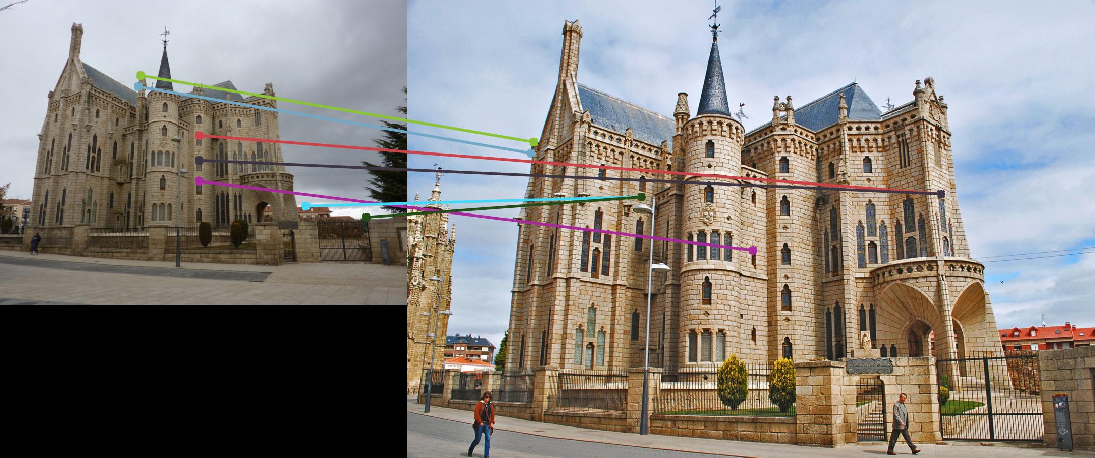
Episcopal Gaudi:

The pipeline performed poorly on the episcopal gaudi image pair. For the full pipeline, there was 0% accuracy. Using the ground truth interest points, there was only 8% accuracy. This is likely because of the difference in both illumination and scale between the two images. The interest points we find are very dependant on scale, so it seems that the interest point finder does a poor job of finding image features in the left image that correspond to image features in the right image. In addition to this, it is clear by looking at the results from the ground truth interest points that the SIFT-like feature descriptor used here is not scale invariant, and so there are poor results even when good corresponding interest points are found in the two images.

Results	Line Visualization