Computer Vision Project

Project 2: Local Feature Matching

The project aims to implement an algorithm to detect certain features of interest and match them across multiple images. First, interest points are found in the two images to be matched using the Harris corner detection algorithm. Then, a 128 dimension feature vector is formed for each feature using a SIFT-like feature desscriptor. The final feature descriptors are then compared for closeness and using a confidence measure, the top 100 most confident matches in corresponding images are shown in the results.

Interest Point Detection

Here, we use points as our objects of interest. Corners are most suitable because they are less ambiguous to detect across multiple images, as they have gradients in multiple directions. For finding corners, the square of image derivatives in both directions is taken to form a matrix M at each pixel. The 'cornerness' of that pixel is then calculated using the relation:

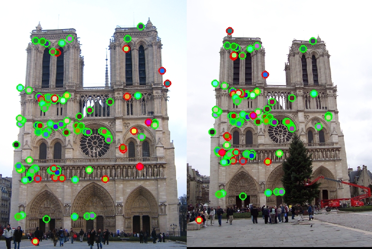
Here, the parameter α is a constant whose value can be tweaked to get different results. The pixels with a cornerness value above a certain threshold are then found and non-maximal suppression is applied. In this case, I found connected components using bwconncomp, found the centroid of each connected component and removed the rest of the points from the corner list. The figure below shows the output of the corner detection function for α=0.04 and a threshold value of 0.5 on the Notre Dame pair.

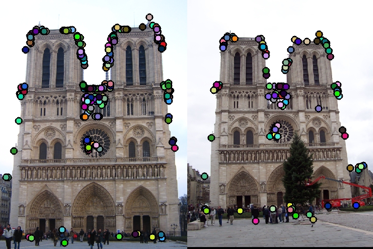
In the actual code, I used a threshold which gave a little more than a thousand interest points (a value of 0.02 for the Notre Dame pair).

Feature Description

The coordinates of the detected features are then passed to the get_features function. Here, a feature_width x feature_width region around the feature is broken down into 16 cells and the gradients inside each cell are split into 8 bins depending on their direction. These 8 numbers for each cell are then concatenated to obtain the final 128-dimension vector. The following code snippet does this:

%% Feature descriptor
% Form feature_width/4 x feature_width/4 cells.
for j=1:feature_width/4
    for k=1:feature_width/4
        for l=-4:3
        	% Binning. The if-else is to handle the discontinuity from -180 to 180 deg (-4 to 4 since I divide by 45).
            if l~=-4
                [r,c]=find(gdir(4*j-3:4*j,4*k-3:4*k)>l-1 & gdir(4*j-3:4*j,4*k-3:4*k)<l+1);
            else
                [r,c]=find(gdir(4*j-3:4*j,4*k-3:4*k)>l+7 | gdir(4*j-3:4*j,4*k-3:4*k)<l+1);
            end

            % Sum up all gradient magnitudes lying along close to direction (l*45) degrees.
            for m=1:size(r)
                features(i,8*feature_width/4*(j-1)+8*(k-1)+l+5)=features(i,8*feature_width/4*(j-1)+8*(k-1)+l+5)...
                						+ 0.5*gmag(c(m),r(m));
            end
        end
    end
end

Finally, as mentioned in Szeliski, I normalised the feature vector, clipped the values above 0.2 to 0.2 and renormalised it (some more details in the Observations section).

Feature Matching

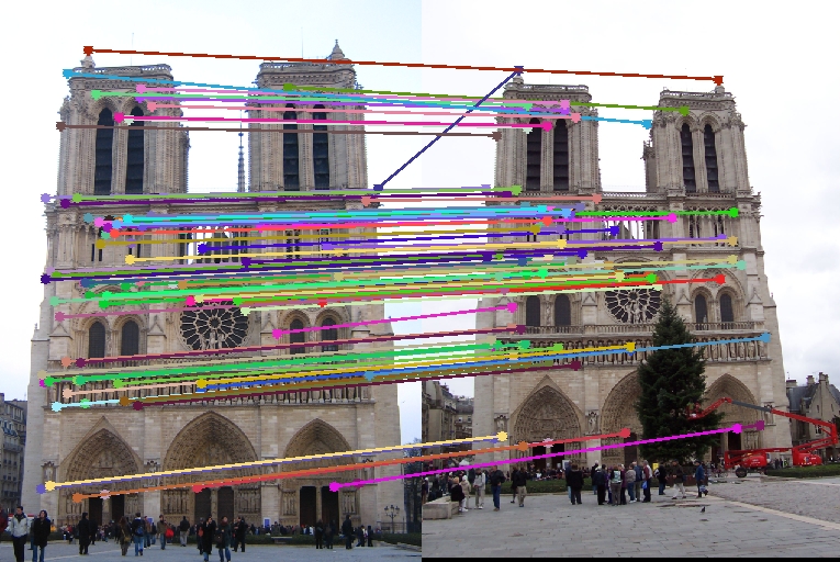
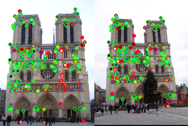
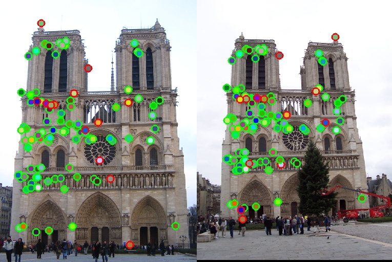
Feature matching using pdist2 was done to find the closest neighbours.Confidences were found by taking the ratio of distances between the nearest and second nearest neighbour--a ratio close to 1 would mean the given feature in image1 has multiple likely matches in image2--and then the features were sorted by confidence. The top 100 matches were taken and then mapped for the two images using the visualisation function provided with the skeleton code. A sample result obtained is shown below:

Observations

Feature Width: The feature_width parameter seems to most heavily affect the accuracy of the obtained features. Below is a table showing the outputs obtained for different feature sizes. Clearly, choosing a larger window leads to much more accurate feature matches at the cost of time and number of computations.

Feature Size 16 20 24 32

Accuracy 76 % 80 % 84 % 89 %

Output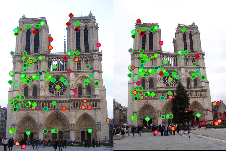
Blur: The amount of blur applied before interest point detection and feature detection also affects the accuracy of the respective steps. During interest point detection, a larger blur seems to decrease the accuracy. On the other hand, there seems to exist an optimal value of blur which needs to be applied to the image before finding gradients for feature description (cutoff_freq = 3 for Notre Dame). Too low and high blurs reduce the accuracy of these steps.
Thresholds: The value of α used during interest point detection step also changes the output accuracy, as shown in the table below. Also, the cutoff threshold for obtaining corners seems to be unusually low in my case. I needed a threshold of 0.02 to obtain 1000+ interest points.

α 0.04 0.05 0.06 0.08

Accuracy 84 % 85 % 84 % 83 %
Clamping the feature vector entries to 0.2 to negate illumination effects did not seem to affect the accuracy for Notre Dame. Reducing this value to 0.15 didn't change anything either, but with a value of 0.1, the accuracy reduced by 2%.
Binning Weights: Using a simple binning method which counts the number of entries in the bin instead of using gradient magnitudes also gave a reduced accuracy by 2%. I also tried weighting the magnitudes depending on how far the gradient direction is from that bin's angle (i.e. a value of 50° would add (1-5/45)*gmag to the 45° bin and (5/45)*gmag to the 90° bin) but this seemed to give a lower accuracy as well, so I finally settled on distributing the gradient magnitude equally to the two closest bins.
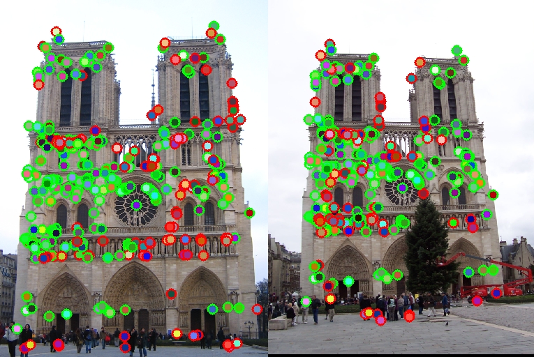
Mapping for Feature Matching: During feature matching, it seemed intuitive to set the distance of the obtained match with the remaining features as Inf to avoid many-to-one correspondences (see figure below).
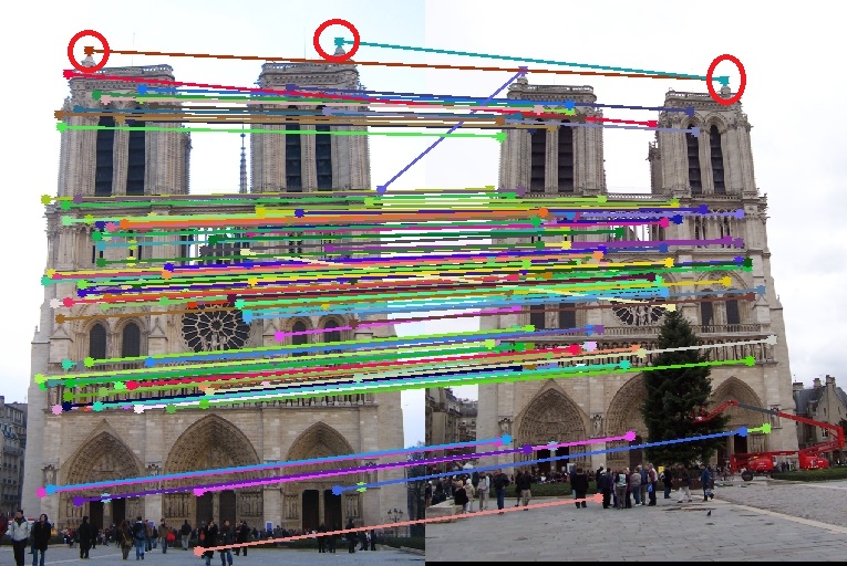
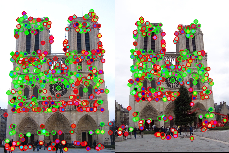
This is not obvious because the order in which we process the matches might affect which features we set to infinity and actually make us miss out on a true match. In practice, up to the first 100 matches, doing this improves the accuracy from 84% to 87%, but if we want a higher number of matches, it reduces it.
Accuracy across number of matches: Summarised in the table below:

No.of Matches 100 150 200 300 500

Accuracy 84 % 81 % 76 % 67 % 51 %

Output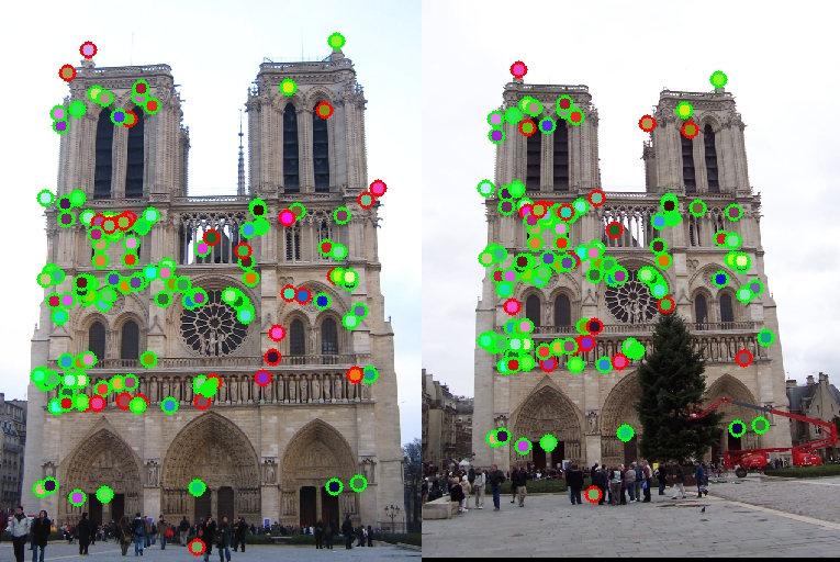
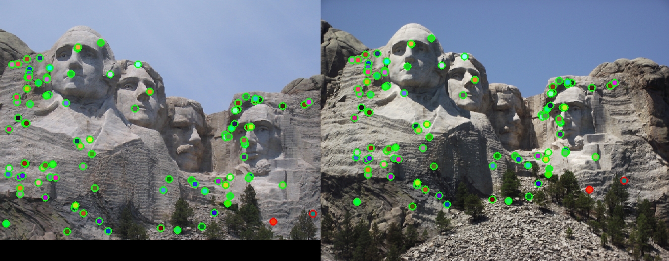
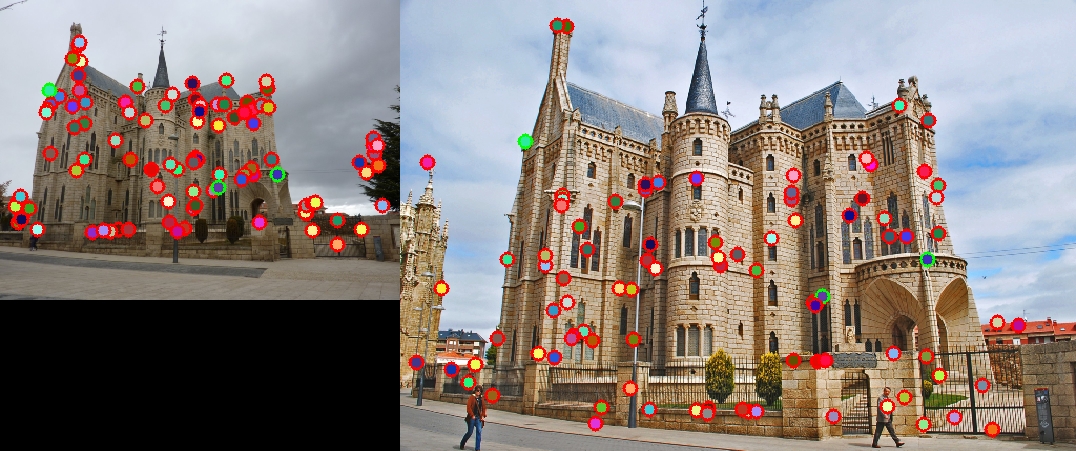
Comparison across images: the accuracy obtained for Mount Rushmore was unexpectedly high (98%). On the other hand, Episcopal Gaudi seems to perform very poorly (3%) accuracy! This is not unexpected because of the extreme difference in the scales of the latter pair. The results obtained for the two pairs are also shown below.