Project 2: Local Feature Matching
Introduction
In this project,we need to implement our own version of SIFT algorithm. More specifically, we implement get_interest_point function to detect interest points, get_features function to capture local descriptor, and match_features function to match_features from image 1 to image 2.
Some details about my algorithm
For match_features function, I use pdist2 to compute the euclidean distance between each features from image 1 and each features from image2, then sort the distances, find the smallest and second smallest distance, and then compute the ratio. For get_features, I build the histogram for each 4*4 cell: check the gradient direction for each pixels and add corresponding value. I add 2 to corresponding bin if the gradient magnitude is greater than 1, add 1 if the value is not greater than 1; it turns out that the result is better than that from adding the gradient magnitude to the histogram. For get_interest_points function, I calculte the harris corner score, and for each 4*4 block, find the maximum score within that block. If the maximum score is greater than threshold, I will keep it as an interest point.
Results of my algorithm
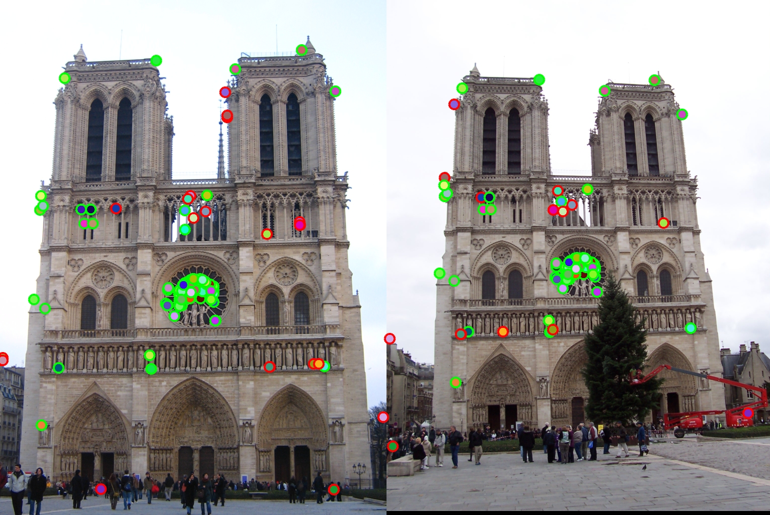
Results of Image Patch and Cheat Interests Point
This results is from using the image patch and cheat_interests_point function.The accuracy is 55%.
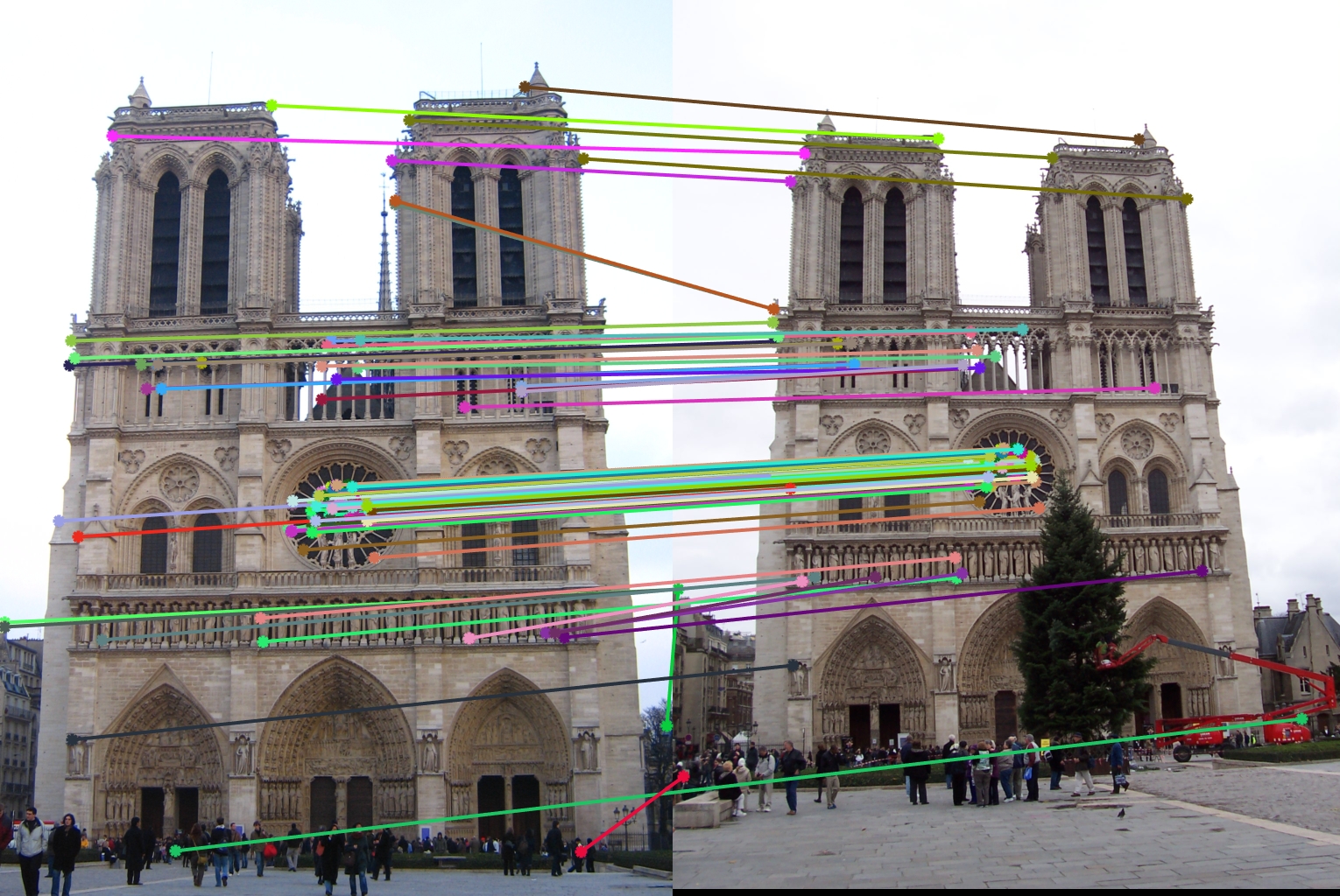
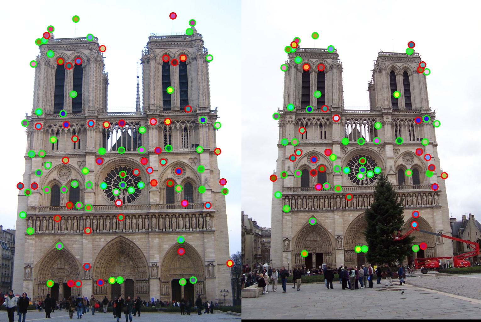
Results of SIFT-Like Features and Harris Corner of Notre Dame
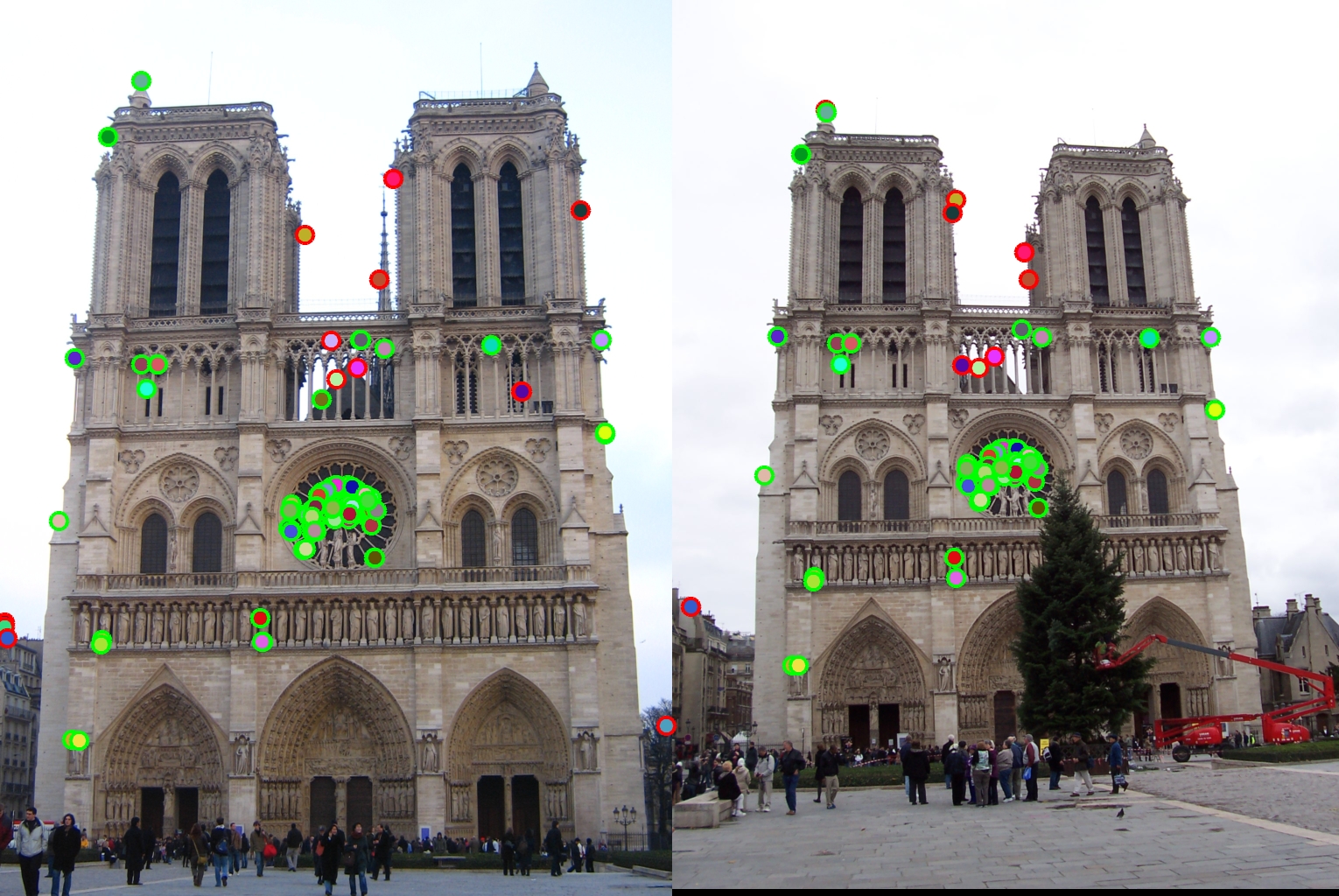
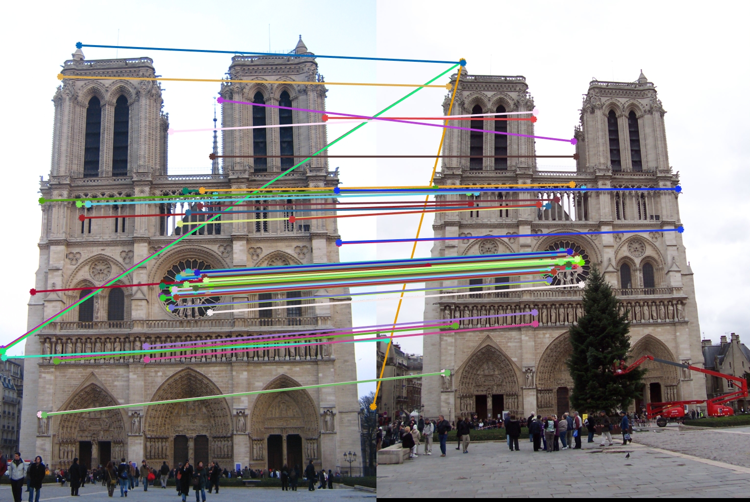
After implementing the SIFT-Like features and harris corner, the accuracy increases to 86%. We can see from ths vis_arrow.jpg that most interest points get matched correctly.
There are a few of parameters that I can tune. For example, the threshold of harris corner score, I find that 0.1 will givethe best accuracy. If I change it to 0.08, then the accuracy will drop below 50%.
Results of SIFT-Like Features and Harris Corner of Other Pairs
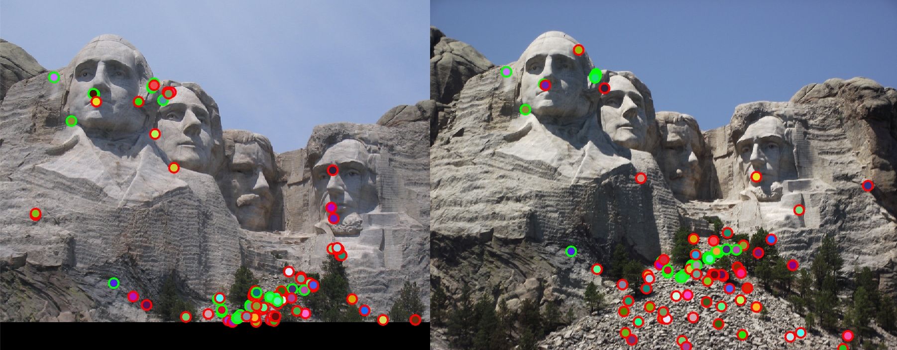
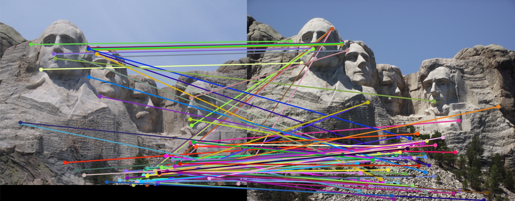
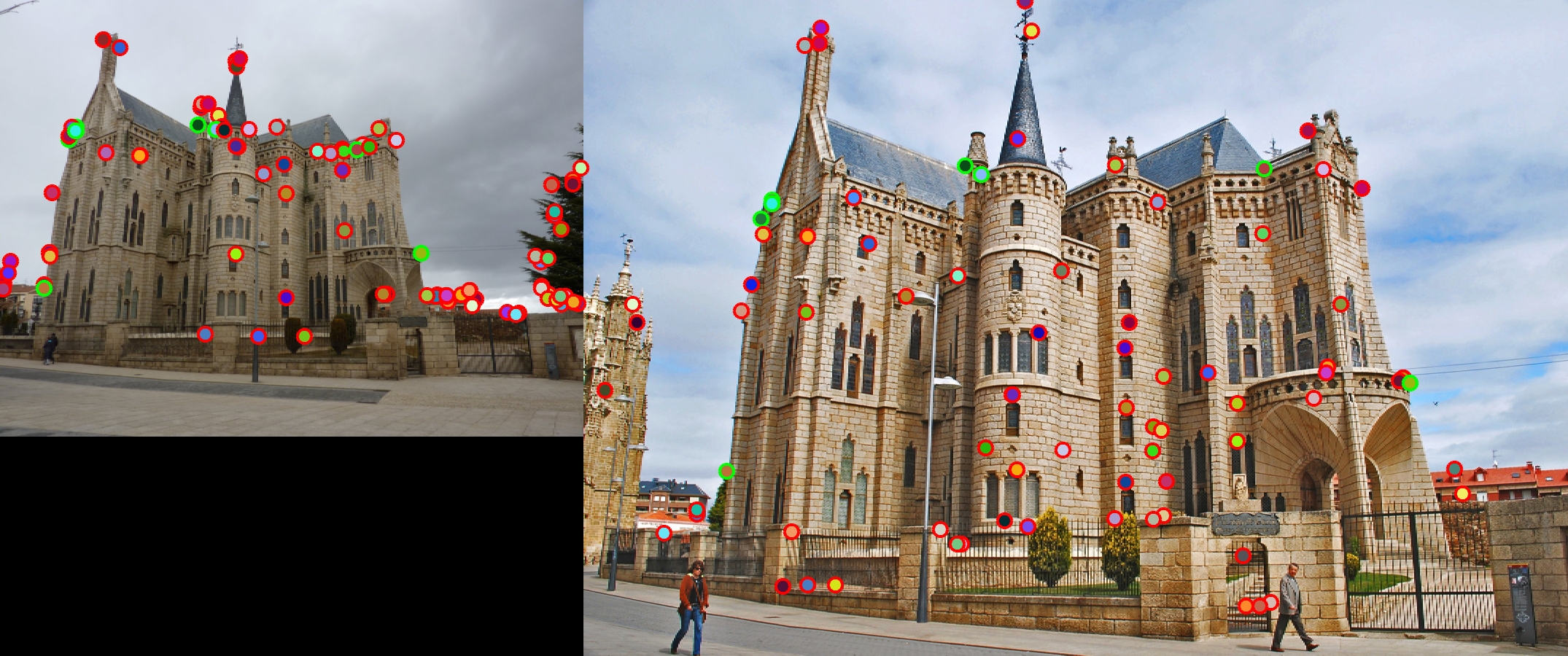
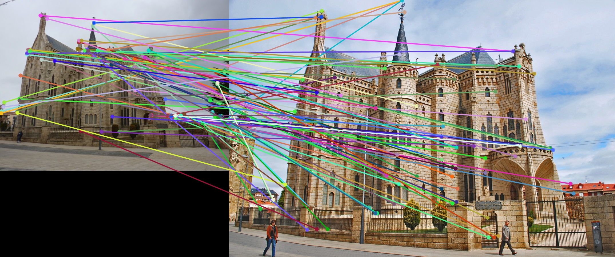
On the other hand,the accuracy for Mount Rushmore and Episcopal Gaudi is very low. The accuracy for Mount Rushmore is 33%, and the accuracy for Episcopal Gaudi is 10%.
Extra Credit
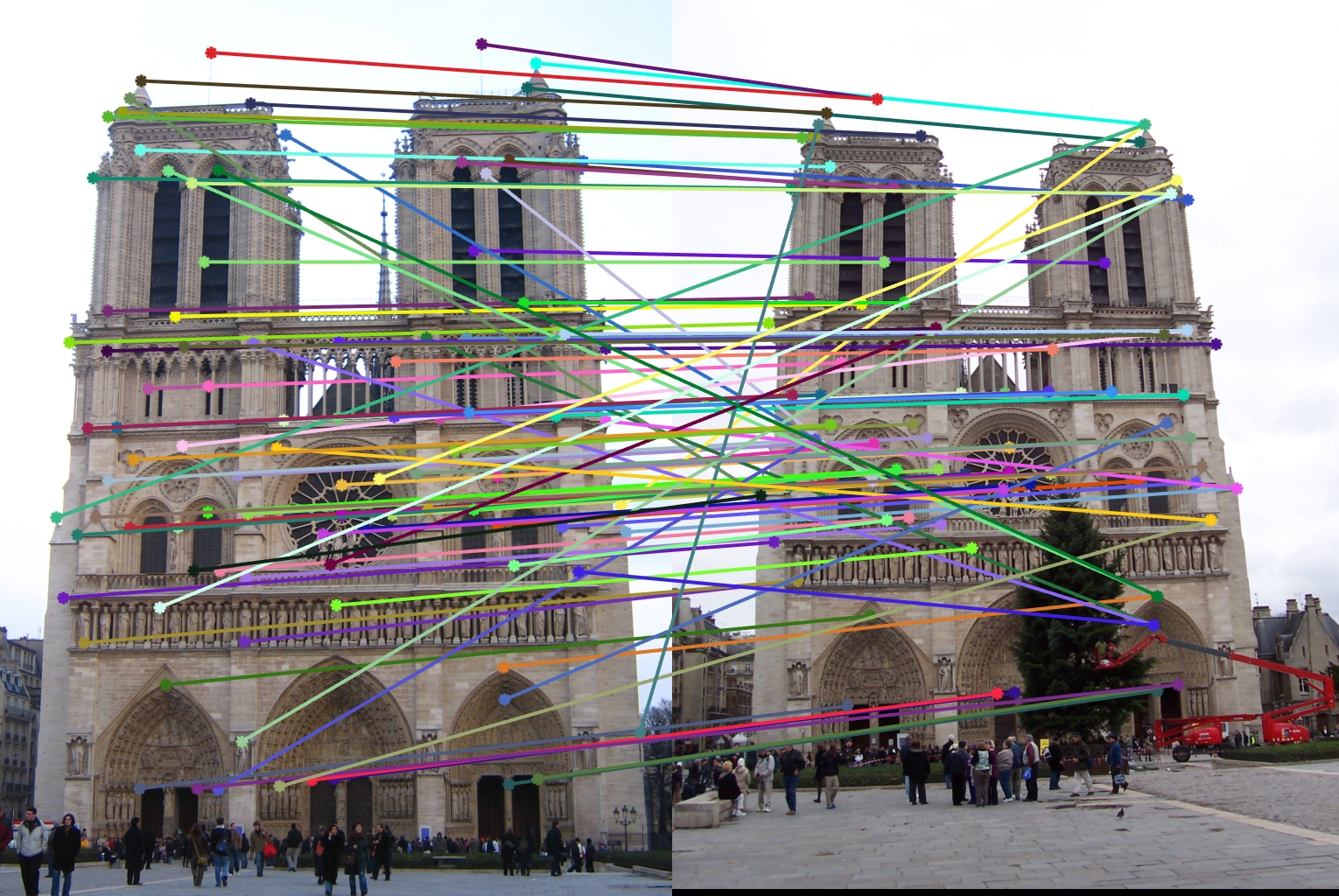
For this project, I also use the PCA to create low dimensional descriptor. I download 20 random images from Internet (see pictures in folder PCA). In build_my_pca function, for each of these 20 images,I get their interest points and corresponding SIFT-Like descriptors, and concatenate all descriptors into a large matrix. Then I computed the PCA basis based on these descriptors and return the PCA basis to a matrix. (One thing to note is that in the get_feature step, I don't do the feature matrix normalization because that will give us a matrix with NaN in PCA computation.I guess the reason is that the value in feature matrix after normalization is very very small, so when we do the feature matrix multiplication, matlab will return NaN). In proj2.m, first call the function build_my_pca to compute the "universal basis" so that we don't have to compute the basis every time we have new images. After we have the 128-dimensional features, we can use the PCA basis to reduce it to 32 dimensions. The elapsed time of matching algorithm before PCA is 0.743398 seconds; the elapsed time after performing PCA is 0.257480 seconds. Since 32 dimensions is 1/4 of 128 dimensions, we should expect the running time of matching algorithm will be 4 times faster with PCA, but the running time with PCA is only 3 times faster than that without PCA. The accuracy after using PCA is not too bad. The accuracy only drops from 86% to 78%, which is reasonable as we only use 32 dimensions of data.
Results using PCA