Project 2: Local Feature Matching
Introduction
This project's goal was on implementing a version of the scale invariant feature transform (SIFT) pipeline similar to that implemented by David Lowe. The SIFT pipeline consists of three major steps:
- 1) Interest point detection
- 2) Feature transformation for each interest point
- 3) Feature matching between images for corresponding points
Component 1: Feature Matching
I first implemented the feature matching between images for corresponding points. Each interest point in both images is represented by 1 x 128 dimensional feature vector, a description of the interest point based on x and y gradient and orientation. Given an interest point k in one image, a similarity metric can be computed for all interest points in the second image. The similarity metric used was the Euclidean distance (L2 norm) between points. However, when just the nearest neighbor is computed, the accuracy for Notre Dame is 78%. Instead, I implemented the nearest neighbor ratio metric as mentioned in the assignment. The nearest neighbor ratio computes the ratio of the nearest neighbor / second nearest neighbor. Rather than sorting the neighbors, I implemented the nearest neighbor ratio by obtaining the nearest neighbor, removing it from the vector, and then taking the nearest neighbor again. With this computation, the accuracy is improved for Notre Dame to 90%.
|
Notre Dame Nearest Neighbor Ratio, Accuracy = 90% for 100 matches. Notre Dame Nearest Neighbor, Accuracy = 78% for 100 matches 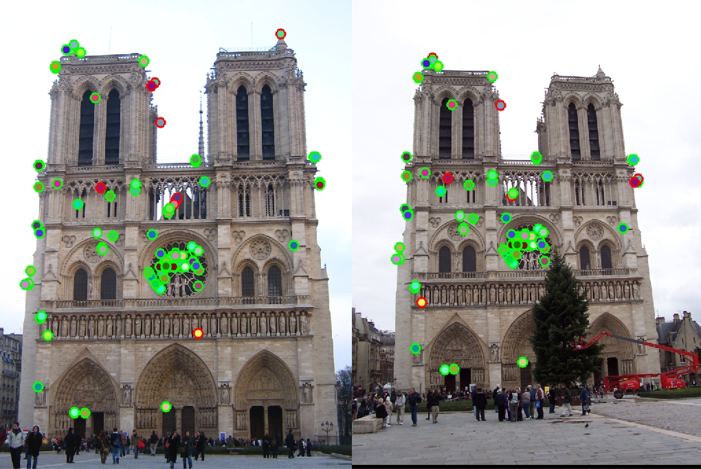
|
Component 2: Feature Transformation
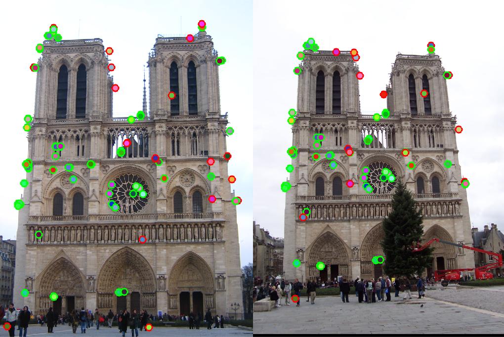
For the second part of the pipeline, I computed SIFT-like features for a set of interest points of an image. According to Lowe's paper the SIFT pipeline is partially inspired by human vision, since neurons in the V1 cortex fire when light is at a particular orientation and gradient. To compute the gradient of the image, I applied a 3x3 x and y oriented sobel filter via convolution. For each interest point, I obtained a 16 x 16 pixel image patch surrounding the patch. I further divided each patch into 16 4x4 cells. Each 4x4 cell of the image has a x-sobel image and a y-sobel image. I computed the orientation of the gradient for each pixel in the 4x4 cell by taking the inverse tan of y-gradient/x-gradient. One small implementation issue I encountered was that because four quadrant inverse tan maps from -pi to pi, I shifted all negative orientations by 2*pi. I computed the magnitude of the gradient of each pixel by computing the L2-norm of the x and y gradient, and I binned the magnitudes based on orientation (8 bins). 16 cells * 8 bins result in the 128 feature space vector for an interest point. Normalization of the feature space and exponentiation by a factor less than 1 significantly improved accuracy. The reason I believe the exponentiation helped is that points that appear far away from each other in the feature space due to noise are actually corresponding points, so exponentiation by 0.4 versus 1 improved accuracy from 84% to 90%.
|
Notre Dame Exponent 0.4, Accuracy = 90% for 100 matches. Notre Dame Exponent 1.0, Accuracy = 84% for 100 matches
|
Component 3: Interest Point Detection
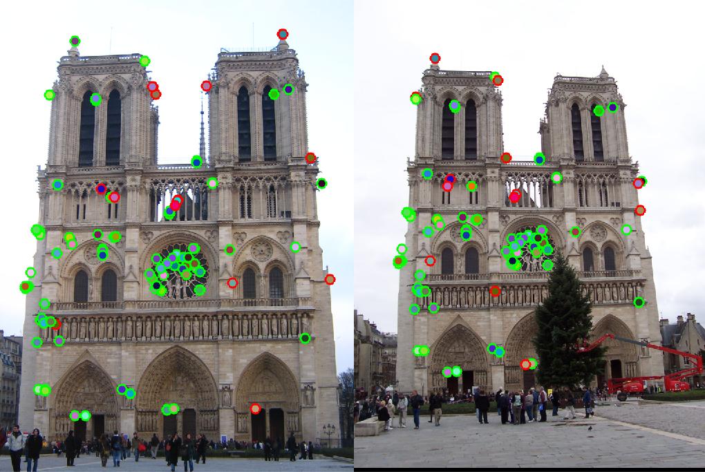
The last part of the pipeline I implemented, but is actually the first step in my SIFT-like pipeline was identifying interest points. I implemented the baseline Harris-corner detection algorithm. I identified interest points by computing x and y derivatives of the image. This was done by convolving the image with x and y Gaussian derivative filters. Then I computed the x^2, xy, and y^2 derivative components, and obtained R values as specified by the Harris corner algorithm for each pixel: R = det(H) - k*trace(H)^2. k was chosen to be 0.05, as mentioned in the slides and literature. I implemented non-maximum suppression by iterating through distinct 6x6 blocks and identifying the maximum local point. I then suppressed all R values less than 0.05. Another implementation detail was that I removed interest points near image boundaries, as they are hard to handle and typically not actually relevant interest points. One important parameter that affected my the SIFT implementation's performance was the size of the sliding window used. This is likely because my implementation of SIFT based on the assignment is not scale-invariant. In addition, the sliding window size impacted the number of interest points identified. When using a sliding window of size 16x16, I obtained ~1000 interest points and the accuracy for Notre Dame was 73%, but with a 6x6 window I obtained ~4000 interest points and the accuracy was 90%. However, smaller sized windows such as 5x5, deteriorated accuracy to 83%. This seems to indicate the appropriate scale of salient interest points in Notre Dame were 6x6.
|
Notre Dame Window Size 6x6, Accuracy = 90% for 100 matches. Notre Dame Window Size 16x16, Accuracy = 73% for 100 matches

|
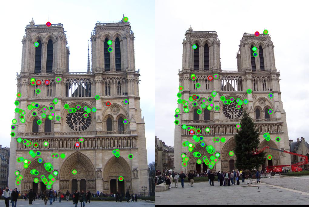
I was still not appeased with the current performance of the SIFT-based pipeline that I implemented. Most interest points found were in high contrast regions in Notre Dame, such as the center window of Notre Dame. I decided to implement adaptive non-maximum suppression (ANMS). Similar to the nearest neighbor distance ratio improvement, the ANMS improves the identification of interest points, and makes sure they try to cover more broadly the image of interest. With ANMS implementation (the best interest point in sliding window is at least 5% better than the next highest interest point), accuracy improves from 90% to 95%, and the interest points for the image cover the image more than previously.
The next thing I was not satisfied with was the run time of my implementation of the algorithm. So, as recommended by the assignment, I used MATLAB's kd-tree function to create a kd-tree model for my interest points, and then I used the knn function to obtain the nearest neighbors from the kd-tree for a given set of points. The accuracy was maintained, while runtime improved for Notre Dame from 94.455386 seconds to 57.900758 seconds.
Component 4: Additional Images
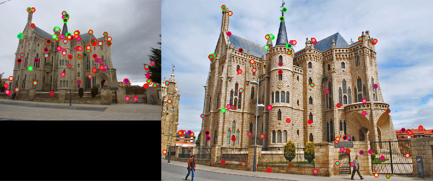
Below are images when the same SIFT pipeline (with same parameter values) are implement to the two other images with ground truths. When applied on Mount Rushmore, accuracy of 98% percent is achieved. When applied to Episcopal Gaudi, accuracy of 16% is achieved. This poorer accuracy may be attributed to the significant difference in scale between the images.
|
Mount Rushmore, Accuracy = 98% for 100 matches. Episcopal Gaudo, Accuracy = 16% for 100 matches 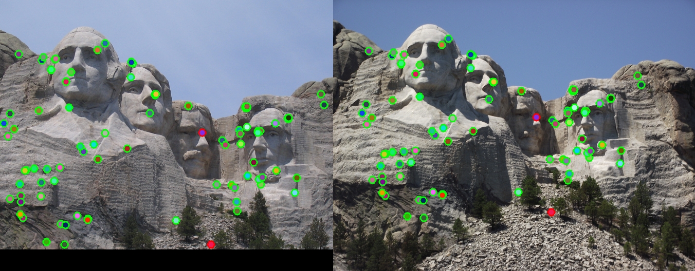
|
Component 5: Conclusion
Conclusion: By first identifying interest points using Harris corner detector, creating a feature vector for each interest point, and matching corresponding features using the nearest neighbor ratio, a basic SIFT pipeline was implemented.