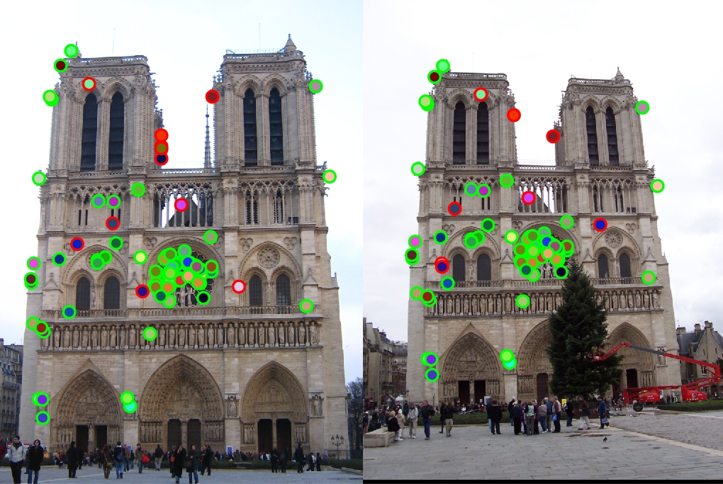
The top 100 most confident local feature matches from a baseline implementation of project 2. In this case, 93 were correct (highlighted in green) and 7 were incorrect (highlighted in red).
In this assignment, we create a local feature matching algorithm using SIFT-like techniques. The pipeline is a simplified version of the famous SIFT pipeline. The matching pipeline is intended to work for instance-level matching -- multiple views of the same physical scene.
The pipeline consists of the following three major steps:
- Interest point detection
- Local feature description
- Feature matching
Interest Point Detection
For this, we use Harris corner detectors to find interest point. An interest point is a point in an image which has a well-defined position and can be robustly detected. Here, we use corners as interest points. A corner can be defined as the intersection of two edges. A corner can also be defined as a point for which there are two dominant and different edge directions in a local neighbourhood of the point. To distinctly identify interest points in multiple images, we need corners as multiple points along an edge are not distinguishable.
The algorithm proceeds as follows:
- Get image gradients and calculate second moments at each pixel
- Smoothen the gradient while weighing closer gradients more using a Gaussian 2D filter
- Calculate the Harris score at each pixel
- Apply non-maximum suppression and threshold the Harris score
- Remove interest points near image boundary
- Return interest points
The code for the algorithm is shown below:
function [x, y, confidence, scale, orientation] = get_interest_points(image, feature_width)

% Get gradients at each pixel
[Ix, Iy] = imgradientxy(image);

% Get second moments for each pixel
Ixx = Ix .* Ix;
Ixy = Ix .* Iy;
Iyy = Iy .* Iy;

% Apply 2D Gaussian filter to smoothen gradients
Gaussian_1d = fspecial('Gaussian', [feature_width 1], 1);
Gxx = imfilter(imfilter(Ixx, Gaussian_1d), Gaussian_1d');
Gxy = imfilter(imfilter(Ixy, Gaussian_1d), Gaussian_1d');
Gyy = imfilter(imfilter(Iyy, Gaussian_1d), Gaussian_1d');

% Caclulate Harris score for each pixel
alpha = 0.05;
har = (Gxx .* Gyy - Gxy .^ 2) - alpha * (Gxx + Gyy) .^ 2;

% Remove low gardients, graythresh makes the threshold adapt to image
threshold = 0.1 * graythresh(har);
har_pruned = har > threshold;

% Non-maximum suppression, finds next highest point in neighborhood
% and checks whether this point is greater than that
nearest_max = ordfilt2(har, 8, [1, 1, 1; 1, 0, 1; 1, 1, 1]);
local_maxima = har > nearest_max;

% Get interest points
har = local_maxima & har_pruned;

% Remove interest points near image boundary
boundary = feature_width * 2;
har(1 : boundary, :) = 0;
har(end - boundary : end, :) = 0;
har(:, 1 : boundary) = 0;
har(:, end - boundary : end) = 0;

% Return interest points
[y, x] = find(har);
After we get the interest points, we proceed to detect local features around those points.
Local Feature Description
For each interest point, we calculate a SIFT-like descriptor vector. This descriptor should ideally be both distinctive and invariant to variations such as illumination, 3D viewpoint, etc. in addition to scale and rotation. However, here we implemented a simplified version which is not invariant to scale and rotation. To compute the local feature descriptor, we borrow ideas from SIFT. Given a feature width, we take a weighted bin count of 8 orientations (binned) per 4x4 sub-matrix to compute the feature vector. We then normalize this feature vector for every point of interest.
The algorithm proceeds as follows:
- Get image gradient magnitudes and directions at each pixel
- Convert gradient directions into corresponding bin from the 8 bins (0:45:360)
- For each interest point, iterate over each cell in 4x4 grid. For each cell, extract subarray of gradient magnitudes and directions. Calculate bin count weighted by gradient magnitudes for each cell. Concatente and normalize to get features for interest point
- Return descriptors for each interest point
The code for the algorithm is shown below:
function [features] = get_features(image, x, y, feature_width)

features = zeros(size(x,1), 128);

% Make feature locations integers and pad image
x = round(x);
y = round(y);
image = padarray(image,[feature_width/2 feature_width/2], 'symmetric');

% Find gradient magnitude and direction
[Gmag, Gdir] = imgradient(image);
% Convert gradient direction into 8 bins
Gdir = min(floor((Gdir + 180) / 45) + 1, 8);

% Iterate over interest points
for i = 1:size(x)
   cnt = 0;
   % Iterate over cells in 4x4 subgrid around interest point
   for cellx_start = x(i) : feature_width / 4 : x(i) + feature_width - 1
       cellx_end = cellx_start + feature_width / 4 - 1;
       for celly_start = y(i) : feature_width / 4 : y(i) + feature_width - 1
           celly_end = celly_start + feature_width / 4 - 1;
           % Extract magnitude and direction bin submatrices
           cell_Gmag = reshape(Gmag(celly_start : celly_end, cellx_start : cellx_end), [], 1);
           cell_Gdir = reshape(Gdir(celly_start : celly_end, cellx_start : cellx_end), [], 1);
           % Compute features for each cell in grid
           for l = 1 : size(cell_Gdir, 1)
               idx = cnt * 8 + cell_Gdir(l);
               % Increments weighted by gradient magnitude
               features(i, idx) = features(i, idx) + cell_Gmag(l);
           end
           cnt = cnt + 1;
       end
   end
   % Normalize interest point features
   features(i, :) = features(i, :) / norm(features(i, :));
end
Feature Matching
Here, we try to match the above computed features across two different images using Lowe's ratio test. Lowe's ration is the ratio of the distance of the nearest neighbor to the point to the distance of the next nearest neighbor to the point. A high ratio means that we have a clear match with little confusion. Then we sort nearest neighbors using this ratio in the ascending order to get the best matches.
The algorithm proceeds as follows:
- For each interest point, get ratio of distance of the nearest neighbor to the point to the distance of the next nearest neighbor to the point. This involves computing the distance to the two nearest neighbors. We use the kd-tree implementation in Matlab to compute these distance for faster computation.
- Sort nearest neighbors in ascending order according to value of Lowe's ratio
- Return best match for each interest point along with confidences in order from most confident to least confident
The code for the algorithm is shown below:
function [matches, confidences] = match_features(features1, features2)

matches = zeros(size(features1, 1), 2);
matches(:, 1) = 1:size(features1, 1);

% Compute distances to 2 nearest neighbors using kd-tree
[idx, d] = knnsearch(features2, features1, 'k', 2, 'NSMethod', 'kdtree');
matches(:, 2) = idx(:, 1);

% Calculate Lowe's ratio
confidences = d(:, 1) ./ d(:, 2);

% Sort the matches so that the most confident onces are at the top of the list
[confidences, ind] = sort(confidences, 'ascend');
matches = matches(ind, :);
Results
We now demonstrate the results of the pipeline the provided sample pairs. We only evaluate the the top 100 highest confidence matches.
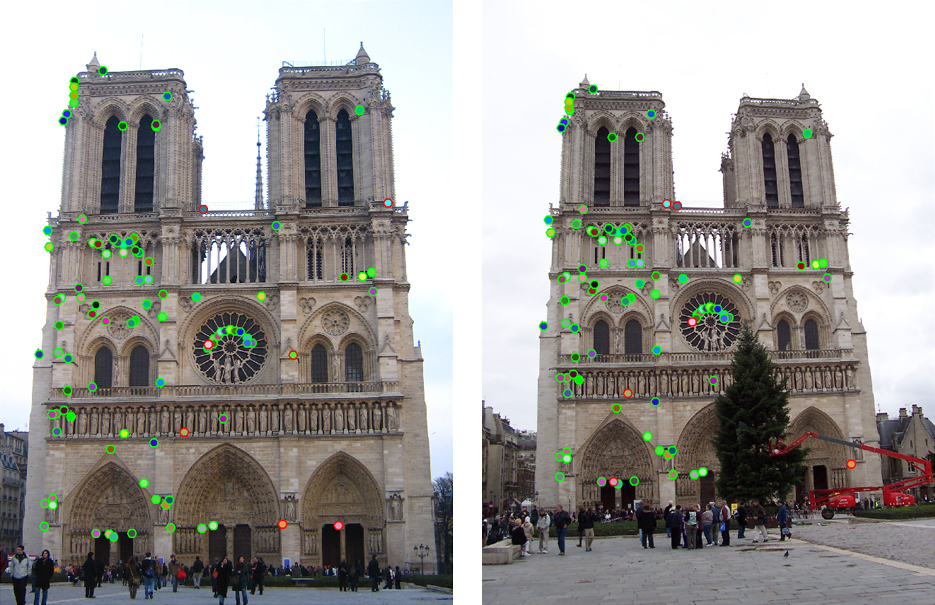
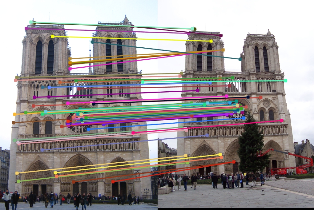
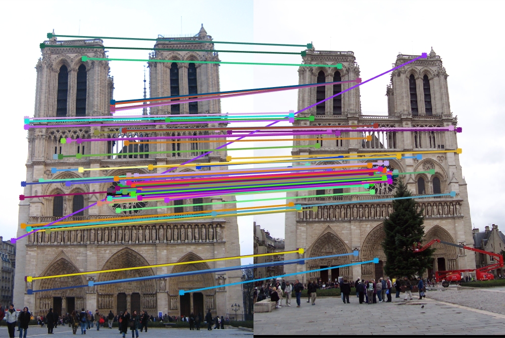
Notre Dame
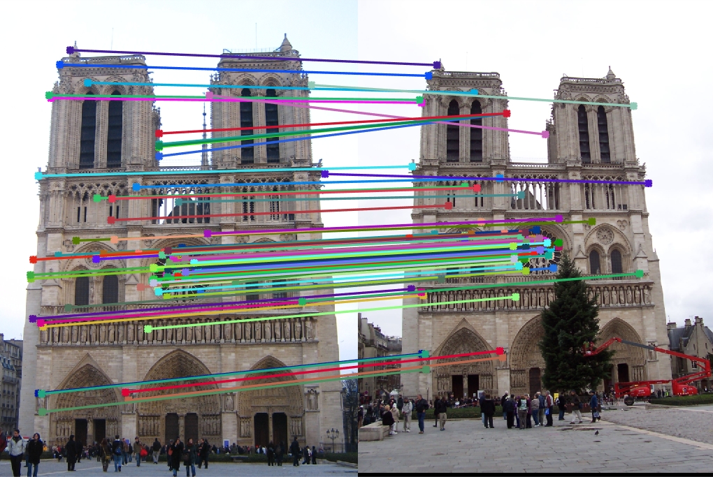
Top 100 matches: 88 good matches, 12 bad matches
The algorithm does well here with 88% accuracy
Mount Rushmore
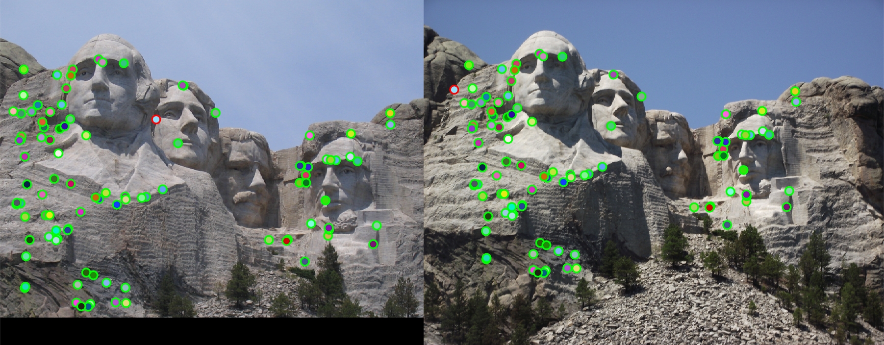
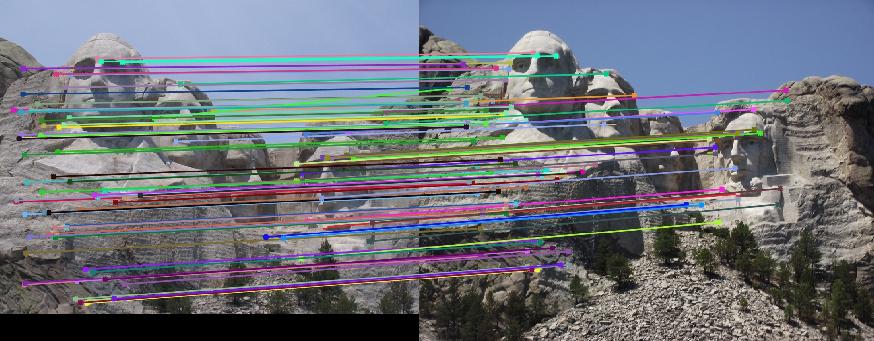
Top 100 matches: 99 good matches, 1 bad matches
The algorithm does extremely well here with 99% accuracy
Episcopal Gaudi
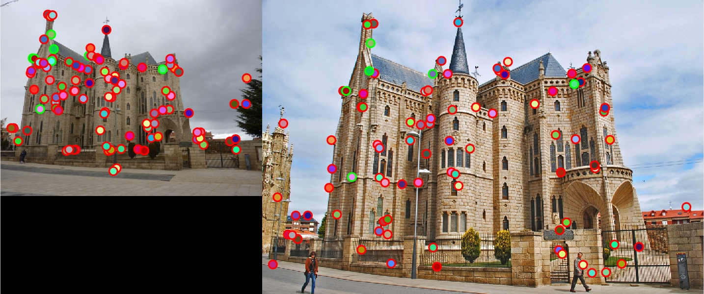
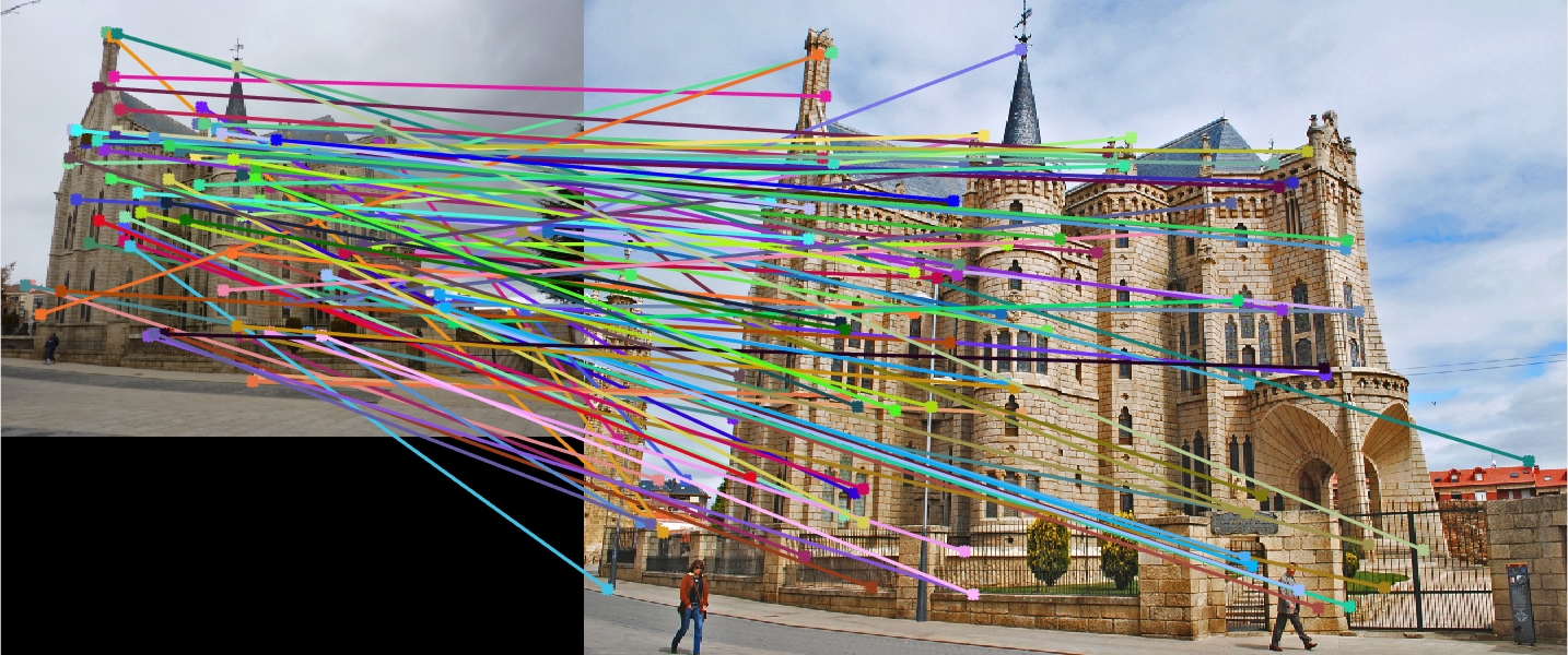
Top 100 matches: 88 good matches, 12 bad matches
Since the images are at different scales and our pipeline is not invariant to scale, the algorithm does poorly with 88% accuracy.
Extra Credit
kd-tree in matching_features
For matching features, we have used the kd-tree implementation in MATLAB to speed up the nearest neighbor search. On average, matching_features takes 1.5 seconds. This is actually slightly slower than calculating the pairwise distance matrix and sorting but the kd-tree is expected to perform better when we work with more features. The relevant code snippet is shown below:
% Compute distances to 2 nearest neighbors using kd-tree
[idx, d] = knnsearch(features2, features1, 'k', 2, 'NSMethod', 'kdtree');
Principal component analysis
We use principal component analysis to reduce the dimensionality of the feature descriptor of each interest point. This would lead to faster matching_features at the cost of some accuracy. For training the PCA transformation matrix and the means for each feature, we used the set of 90 images provided in extra_data. Please note that our implementation requires all these images to put in the folder ../data/all_data without any nesting or subdirectories.
The PCA algorithm was trained as follows:
- For each image get all interest point features and stack them to create a sum_n_features x 128 matrix
- Using MATLAB's pca function compute the means and transformation matrix for the given number of components
- Save the means and transformation matrix for deployment when processing features for a pair of images
The relevant code is shown below:
files = dir('../data/all_data/*.jpg');

feature_matrix = [];
feature_width = 16;

for i = 1 : length(files)
    image = imread(strcat('../data/all_data/', files(i).name));
    image = single(image)/255;
    scale_factor = 0.5;
    image = imresize(image, scale_factor, 'bilinear');
    image_bw = rgb2gray(image1);
    [x, y] = get_interest_points(image_bw, feature_width);
    [image_features] = get_features(image_bw, x, y, feature_width);
    feature_matrix = [feature_matrix; image_features];
end

n_comp = 32;
[coeff, ~, ~, ~, explained,mu] = pca(feature_matrix, 'NumComponents', n_comp);
disp('Explained variance: ')
disp(sum(explained(1:n_comp)));
save('pca_data', 'coeff', 'mu');
PCA was used in get_features_pca to reduce the dimensionaly of each descriptor. We centre the feature matrix around the precomputed means and multiply by the transformation matrix to get the reduced dimensionality feature matrix. The code is shown below:
load pca_data.mat coeff mu;
features = bsxfun(@minus, features, mu) * coeff;
Results
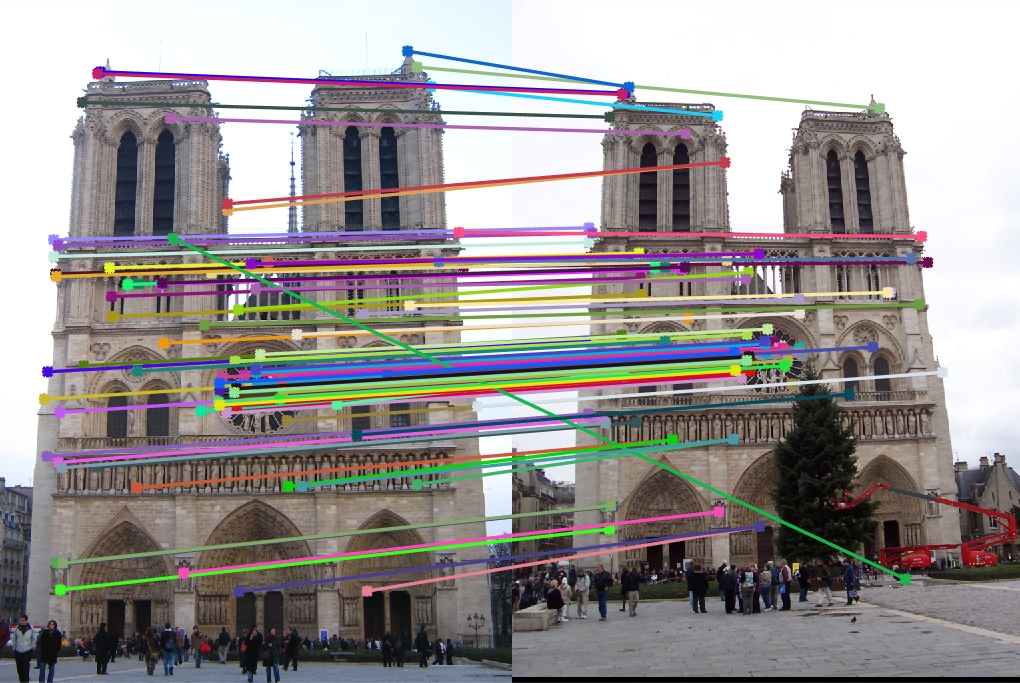
Notre Dame for 64 components
Explained variance: 82.87%
Top 100 matches: 85 good matches, 15 bad matches
There is a slight degradation as accuracy falls from 88% to 86%.
Notre Dame for 32 components
Explained variance: 67.05%
Top 100 matches: 86 good matches, 14 bad matches
There is a slight degradation as accuracy falls from 88% to 85%.
Notre Dame for 16 components
Explained variance: 47.58%
Top 100 matches: 84 good matches, 16 bad matches
There is a slight degradation as accuracy falls from 88% to 84%.
Parameter tuning
We tuned the feature width, the harris score threshold, the graythresh threshold and number of PCA components to find the optimal values. The optimal values were as follows:
- feature_width = 32
- harris_threshold = 0.05 # gradient
- threshold = 0.01 # graythresh
- n_components = 32
We noticed that increasing feature width improved accuracy as features became more distinctive but after a point, the accuracy fell as features became less invariant across images. For Harris score threshold, 0.01 seemed to be the local maxima for accuracy with lower accuracy as we move higher or lower. The same was true for graythesh threshold. For PCA, we tried to balance observed accuracy and explained variance.