Srijan Sood (ssood7)

Project 2: Local Feature Matching

Local Feature Detection and Matching

In Computer Vision, feature detection is the act of identifying image points, curves, or regions that are used to make decisions of some kind. In this project, we identify features that can be used for local feature matching. Feature Matching is the act of finding common features in two images with overlapping content, but possibly different scale, orientation, illumination etc. THis has applications in image alignment (eg. panorama stitching), video stabilization, motion tacking etc.

In this project, a simplified version of the SIFT pipeline was used. The objective was instance-level mathcing (different views of the same physical scene). The algorithm has 3 main components:

1. Interest Point Detection (get_interest_points.m)
2. Local Feature Description (get_features.m)
3. Feature Matching (match_features.m)

Interest Point Detection

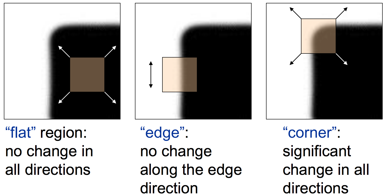
A Harris Corner Point Detector was used to find keypoints. The basic intuition behind the Harris Detector is that sliding a small window over the image causes graident change in different directions. This can be used to detect corners as shifting the window in any direction will result in a large change.

The pseudocode used:

1. Compute the horizontal and vertical derivatives of the image Ix and Iy by convolving the original image with derivatives of Gaussians.
2. Compute the three images corresponding to the outer products of these gradients.
3. Convolve each of these images with a larger Gaussian.
4. Compute a scalar interest measure using the second moment matrix. R = det(M) - alpha x trace(M)^2
5. Find local maxima of responses above a certain threshold and report them as detected feature point locations.

				function [x, y, confidence, scale, orientation] = ...
				         get_interest_points(image, feature_width)

				% small gaussian for blurring
				blur_gaussian = fspecial('gaussian', [3, 3], 1);
				image = imfilter(image, blur_gaussian);
				[dx, dy] = imgradientxy(image);

				gaussian = fspecial('gaussian', [16 16], 1); % larger gaussian
				dx_sq = imfilter(dx .* dx, gaussian);
				dy_sq = imfilter(dy .* dy, gaussian);
				dxdy = imfilter(dx .* dy, gaussian);

				% Harris Corner Detector:
				% 1) Compute M matrix for each image window to
				% get their cornerness scores.
				% 2) Find points whose surrounding window gave
				% large corner response (f> threshold)
				% 3) Take the points of local maxima, i.e., perform
				% non-maximum suppression

				Mtemp = [dx_sq dxdy; dxdy dy_sq];
				M = imfilter(Mtemp, gaussian); % auto-correlation matrix

				% response = det(M) - alpha * trace(M)^2
				det_M = (dx_sq .* dy_sq) - (dxdy.^2);
				trace_M = dx_sq + dy_sq;
				alpha = 0.06;
				response = det_M - alpha .* trace_M .^ 2;

				% Suppress the gradients/corners near the edges of the image
				response(1 : feature_width, :) = 0;
				response(end - feature_width : end, :) = 0;
				response(:, 1 : feature_width) = 0;
				response(:, end - feature_width : end) = 0;

				maximum = max(max(response));
				mean = mean2(maximum);
				threshold = response > (maximum / (1000 * mean)) * maximum;
				response = response .* threshold;
				max_response = colfilt(response, [feature_width/2 feature_width/2], ...
				'sliding', @max);
				response = response .* (response == max_response); % only keep max

				[y, x] = find(response > 0);
				confidence = response(response > 0);
				end

			

Feature Description

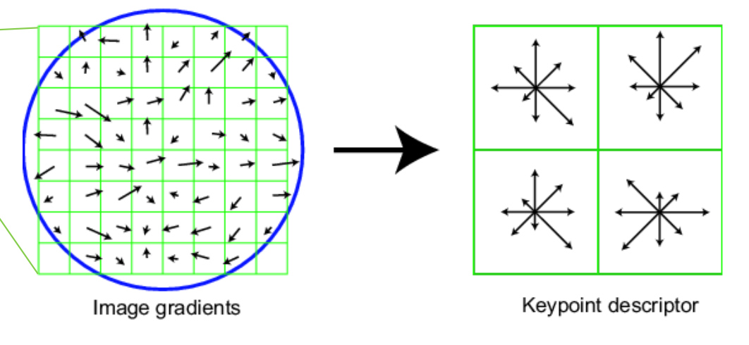
A SIFT-like (Scale invariant feature transform) feature descriptor was used. This works by computing the gradient in a 16x16 window around each pixel. 8 orientation histogram bins are formed for a 4x4 array of graident distributions, hence leading to 128 dimensions. Finally, the features are normalized.

Using SIFT led to a ~30% increase in accuracy as compared to an approach that uses only normalized patches.

				function [features] = get_features(image, x, y, feature_width)

				features = zeros(size(x,1), 128);
				win_rng = feature_width/2;
				bin_angles = -180:45:180;

				for i = 1 : length(x)
					window = image(y(i) - win_rng - 1 : y(i) + win_rng, ...
					x(i) - win_rng - 1 : x(i) + win_rng);

					[Gmag, Gdir] = imgradient(window);
					curr_feature = zeros(1, length(features(1, :)));

					for r = 1:4:feature_width
						for c = 1:4:feature_width

						% A set of bins for each cell
						bins = zeros(1, length(bin_angles) - 1);
						for a = r:r+3
							for b = c:c+3
								direction = Gdir(a, b);
								% Histogram for bins
								idx = find(histcounts(direction, ...
								      bin_angles));
								bins(idx) = bins(idx) + Gmag(a,b);
							end
						end
						% Append this cell to current feature
						append_index = (r - 1) * 8 + ((c * 2) - 1);
						curr_feature(append_index:append_index + ...
						     length(bins) - 1) = bins;
						end
					end
					curr_feature = curr_feature / norm(curr_feature); % Normalize
					features(i, :) = curr_feature;
				end

				end

			

Feature Matching

The Euclidean distance of Image 1 feature vectors to Image 2 feature vectors was calculates. These distances were then used to calculate and store the Nearest Neighbor Distance Ratio (NN1/NN2) where NN1 and NN2 are the distances to the 1st and 2nd nearest neighbors. These ratios were then sorted, and then thresholded. Selecting the threshold as 0.55 gave the best results.

				function [matches, confidences] = match_features(features1, features2)

				num_features1 = length(features1);
				num_features2 = length(features2);

				distances = pdist2(features1, features2); % euclidean difference
				[sorted_distances, indices] = sort(distances, 2);
				scores = sorted_distances(:, 1) ./ sorted_distances(:, 2); % NNDR


				threshold = 0.75; % experiment
				confidences = 1 ./ scores(scores < threshold);
				k = size(confidences, 1); % k x 1
				matches = zeros(k, 2); % k x 2

				matches(:, 1) = find(scores < threshold);
				matches(:, 2) = indices(scores < threshold);

				[confidences, ind] = sort(confidences, 'descend');
				matches = matches(ind,:);

			

Results

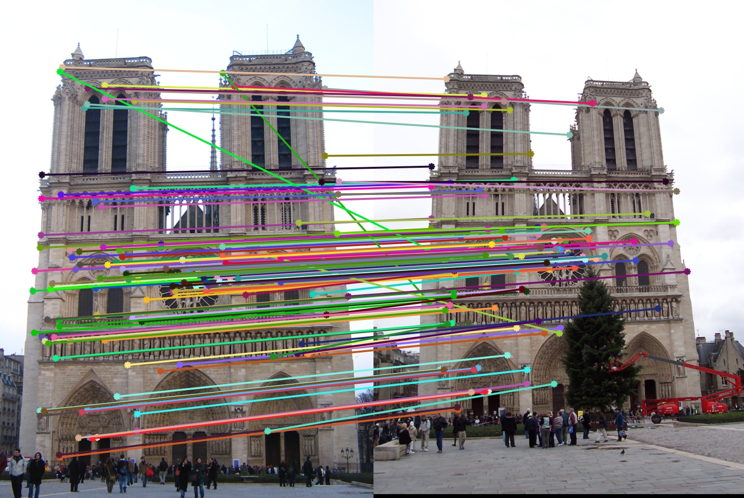
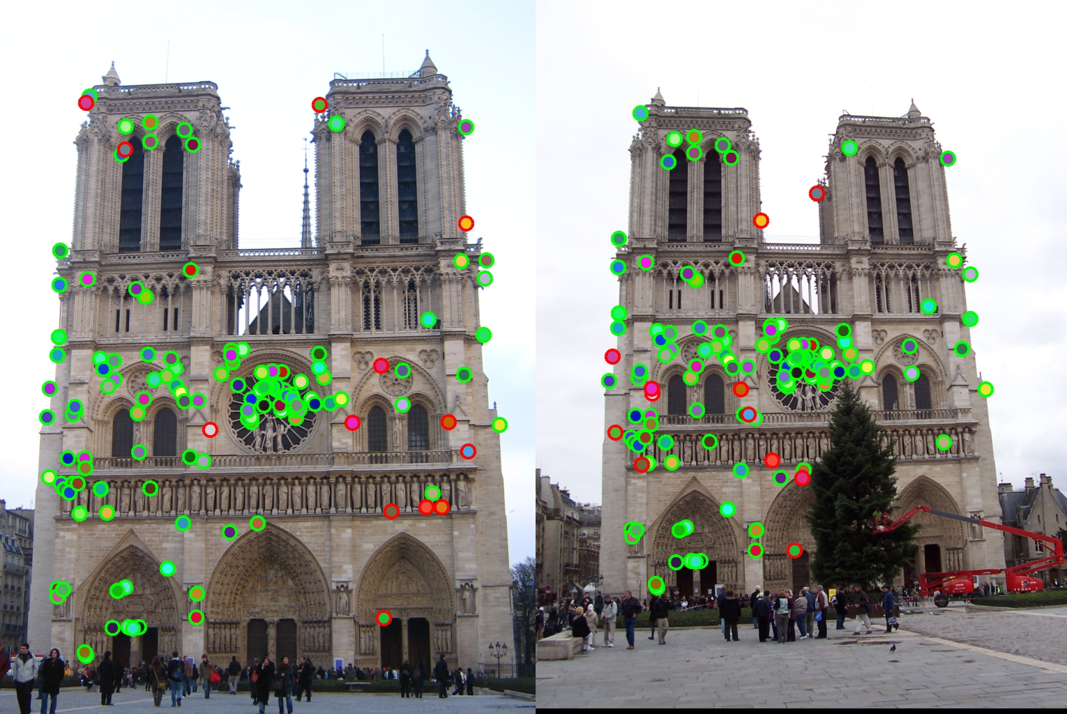
The pipeline resulted in a 91% accuracy on the Notre Dame image pair, with 118 good matches, and 12 bad. The dots with red outlines represent bad matches, and the ones with green outlines represent good.

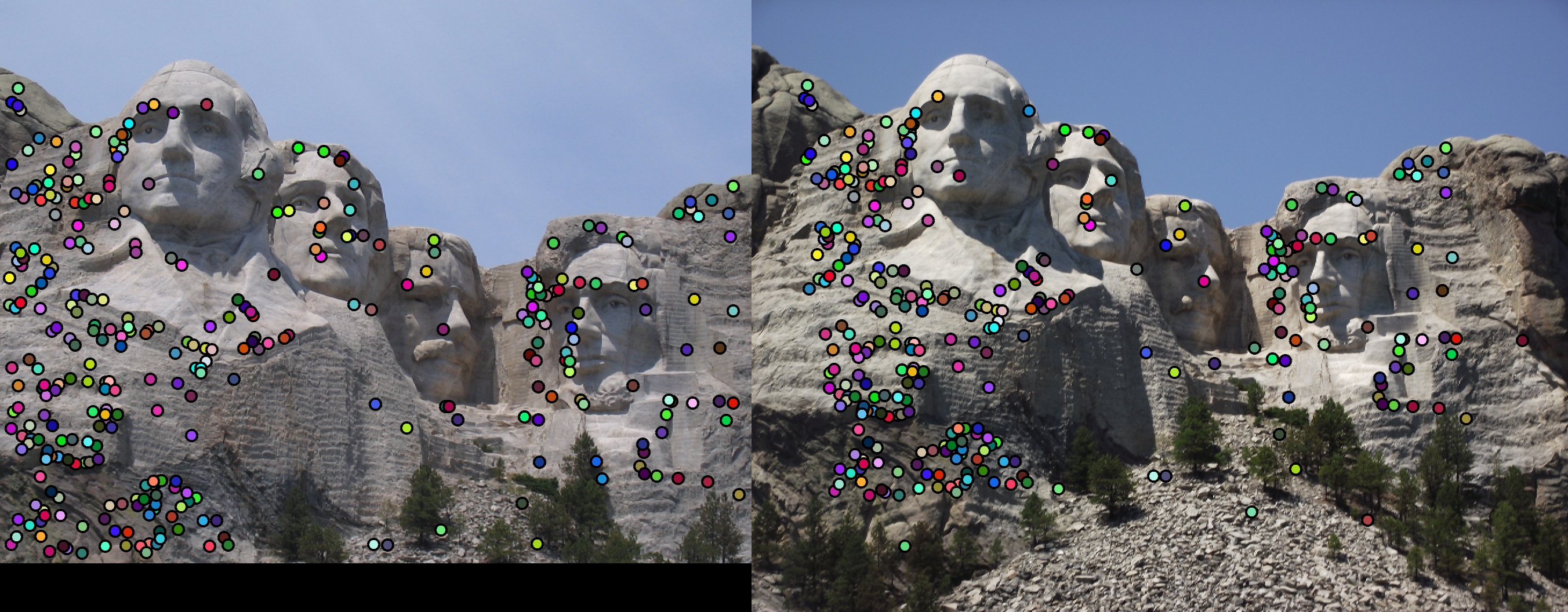
Accuracy for the Mount Rushmore image pair was 89%, with 298 good matches, and 36 bad. Matching dots indicate (good and bad) matches. Outlines (in the second image) represent accuracy.

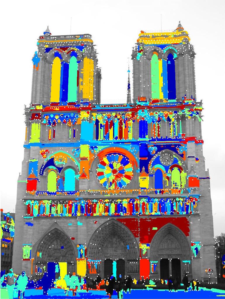
I also wanted to experiment with MSER, and see what regions it highlighted, and how the points chosen by Harris compare. The following is an image of the Notre Dame image with regions highlighted, and Harris Corner interest points marked by tiny white dots.