Project 2: Local Feature Matching
Feature Matching Pipeline
Given two input images A and B, the pipeline:
- Finds interest points for A and B.
- Computes a feature descriptor for all interest points.
- Finds matching features between A and B.
- Visualizes the matching interest points.
Feature Detection
The pipeline uses the Harris Corner Detection algorithm to find interest points for each of the input images. The algorithm finds corners by approximating points where there are large variations in the neighborhood of the point in all directions (vertical and horizontal).
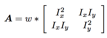
Harris Corner Detection Algorithm
- Compute the directional gradients Ix and Iy for the input image.
- Compute the outer products of the gradients Ix2, Iy2, and Ixy.
-
Convolve each of the outer products with a Gaussian weighting kernel w(σ). Note that the resulting images can be used to form the second moment autocorrelation matrix.
-
Compute "cornerness" for each image pixel (Harris and Stephens 1988).

- Suppress non-maximal values in image H.
- Return coordinates of positive values in image H.
Example Output
Input Image (I). |
Harris Response (H). |
Parameter Tuning
Gaussian Weighting Kernel: Standard Deviation (σ)
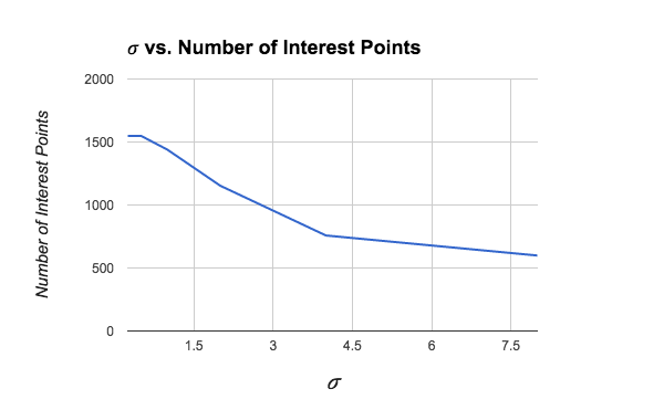
The figure above shows how the value of σ affects the number of interest points detected in the Notre Dame image. A larger value of σ will blur the image gradients over a larger area, producing a smoother correlation surface with fewer local maxima (interest points). A smaller value of σ does not smooth the noise as much, resulting in more interest points detected.
Response Thresholding
Local maxima in the Harris response matrix (H) can be further filtered with thresholding.
| Threshold Value | Number of Interest Points | Accuracy for 100 Most Confident Matches (Notre Dame) |
mean(H) |
1439 | 89% |
mean(H(H > 0)) |
349 | 51% |
mean(H) - std(H) |
1941 | 88% |
Using the mean of all elements (including zeros) in H gave more interest points than using the mean of the nonzero elements in H. Note that the pipeline's matching accuracy suffered when using fewer interest points (high threshold) -- this is because, with more interest points, there are more matches of high confidence (which tend to be accurate). On the other hand, with too many interest points (low threshold), match confidence can degrade because there are too many neighbors in the feature space.
Feature Description
Once detected, the pipeline encodes each interest point into a SIFT-like feature vector. Each feature vector is a concatenation of the gradient orientation histograms for each spatial "cell" in the image patch centered at the interest point.
SIFT-like Feature
- Cut out a square image patch around the given interest point.
-
Compute a gradient orientation histogram for each 4x4 spatial cell in the image patch.
- Each pixel contributes to two nearest gradient orientation bins.
- Contributions are weighted by closeness to the orientation axis.
- Combine the histograms into one feature vector.
Parameter Tuning
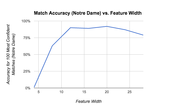
Feature Width
Feature width (measured in pixels) is the length of the square image patch about the given interest point. This pipeline uses a feature width of 16 by default (as described in the original SIFT paper), but is designed to work with any feature width 4k, k = 1,2,3,.... The table below shows the pipeline's matching accuracy for a range of feature widths.
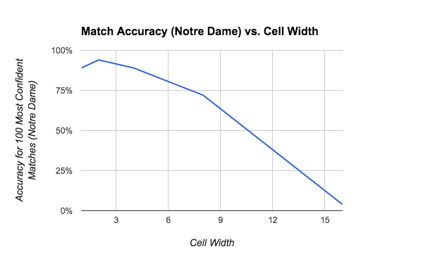
Cell Width
Cell width (measured in pixels) must be a factor of feature width (which is 16 by default). The pipeline uses a cell width of 4 by default. The figure below shows the effect of changing cell width when feature width is held constant at the default value of 16.
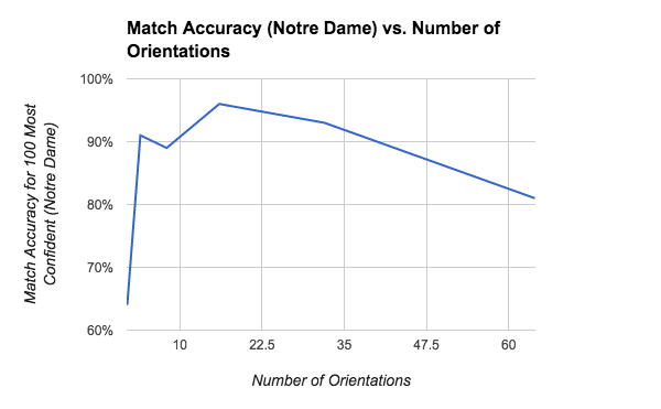
Number of Orientations
The SIFT-like feature builds a gradient orientation histogram with p bins for each cell in image patch of interest. Holding all other parameters constant, the figure below shows the pipeline's match accuracy for a varying number of orientations (p).
Number of Contributions
In a basic SIFT-like feature, each pixel only contributes to the histogram for its own cell. However, this approach is suboptimal because a small shift in the feature window will change the pixels belonging to each cell, resulting in a potentially very different feature vector. To make the feature more invariant to window shifts, I made each pixel additionally contribute to the four adjacent cell histograms. The table below shows the pipeline's matching accuracy when using a single contribution and when using the 4 additional (interpolated) contributions.
| Number of Contributions | Match Accuracy for 100 Most Confident (Episcopal Gaudi) |
| 1 | 5% |
| 5 (interpolation) | 9% |
Feature Matching
With feature vectors computed for each image, the pipeline uses the k-nearest neighbors algorithm to find matches between the input images. For each feature vector a in image A, the nearest neighbor b1 and second nearest neighbor b2 in image B are found using MATLAB's knnsearch function. The nearest neighbor b1 is used as the matching point, and the confidence of the match is given by the ratio (b2 / b1).
Feature Matching Results
Test Image Pairs
After tuning pipeline parameters, the feature matching pipeline was tested on the three image pairs below, and the accuracy was evaluated using ground truth correspondences for the test images.
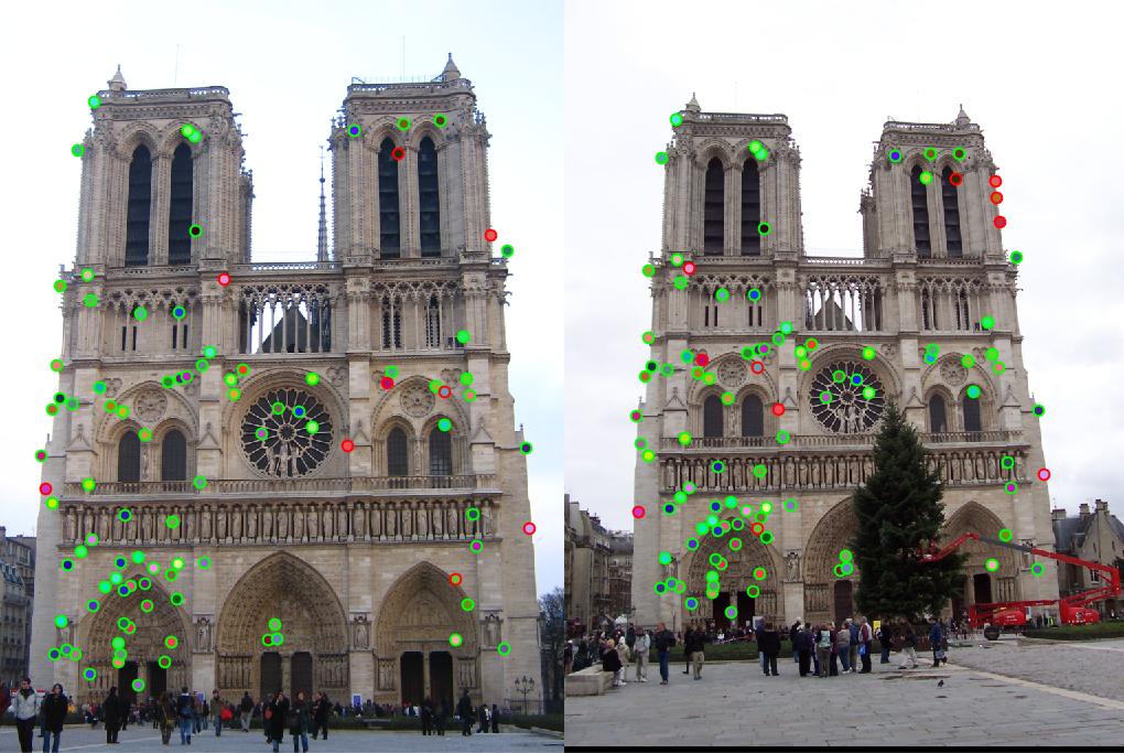
"Notre Dame": 89% accuracy
This image pair is relatively easy because the cameras are calibrated similarly, and the building in the image has many definitive corners/features. The image below shows the matching accuracy for this test case; green points were matched correctly, and red points were matched incorrectly.
Evaluation of 100 Most Confident Matches (89% accuracy).
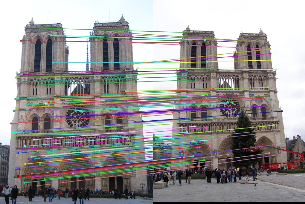
Visualization of matched features.
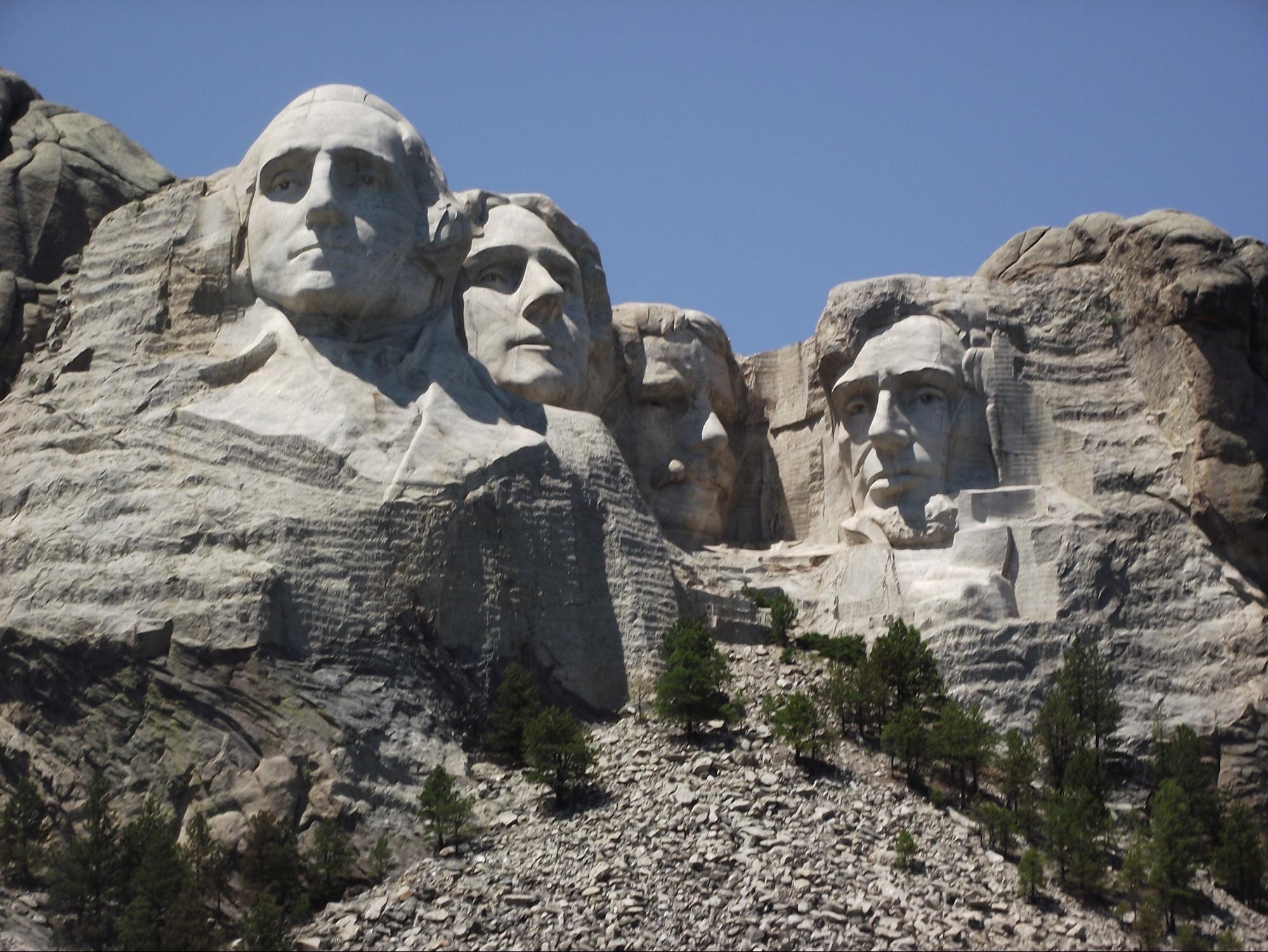
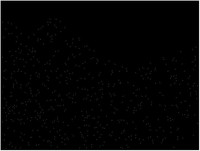
"Mount Rushmore": 100% accuracy
This test case is slightly harder than "Notre Dame", but is still relatively easy due to the similar camera perspectives.
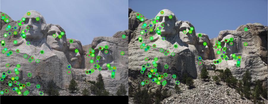
Evaluation of 100 Most Confident Matches (100% accuracy).
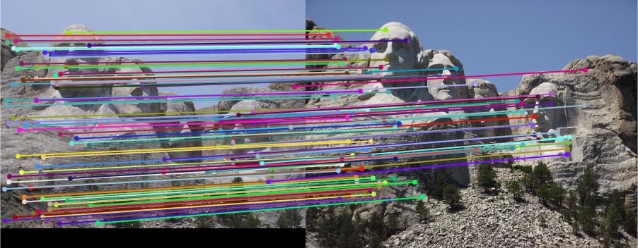
Visualization of matched features.
"Episcopal Gaudi": 9% accuracy
This test case is relatively difficult because the camera perspectives are from slightly different angles, and the images are not the same size. The pipeline computes features using a fixed feature width (measured in pixels), so the feature window about some point (x, y) will contain a "zoomed out" view for the smaller image and a "zoomed in" view for the larger image, resulting in drastically different feature vectors that are unlikely to be matched.
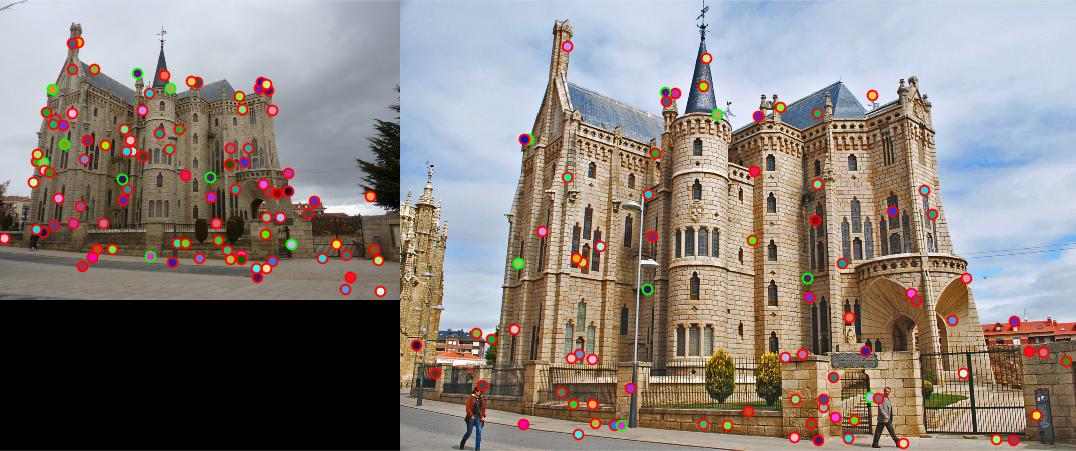
Evaluation of 100 Most Confident Matches (9% accuracy).
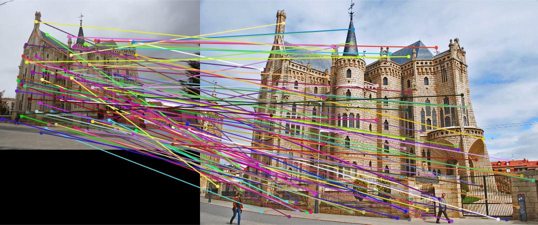
Visualization of matched features.
Additional Image Pairs
The feature matching pipeline was tested on additional image pairs (without ground truth available). Even without an exact evaluation of the matching accuracy, the relative effectiveness can be judged by inspecting the matches visualized in the images below.
"Capricho Gaudi"
This image pair is relatively difficult because the perspectives are different, and the images are not the same size. The image below shows matched features -- there are many incorrect matches, however several distinct features (e.g. top of the tower) were matched correctly. Matching accuracy could be improved by detecting/matching features at multiple scales rather than using one fixed feature size.
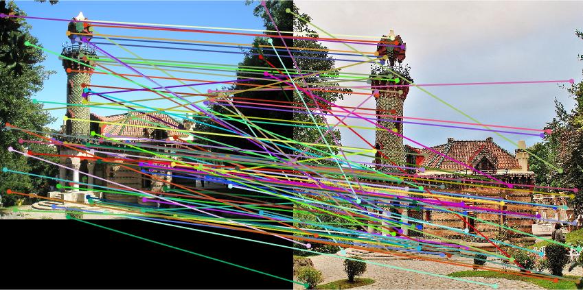
Visualization of matched features.
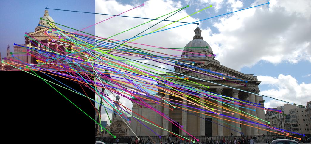
"Pantheon Paris"
There are several image pairs for the Pantheon. The first pair has images of similar scale and perspective, so the matching accuracy is relatively high.
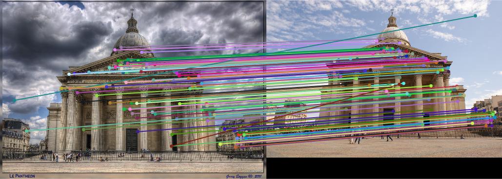
High matching accuracy for similar views of the Pantheon.
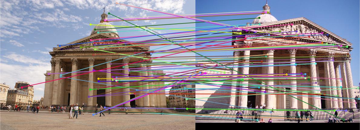
Reduced accuracy for slightly different views of the Pantheon.
Reduced accuracy for Images of Different Scale.