Takuma Nakamura

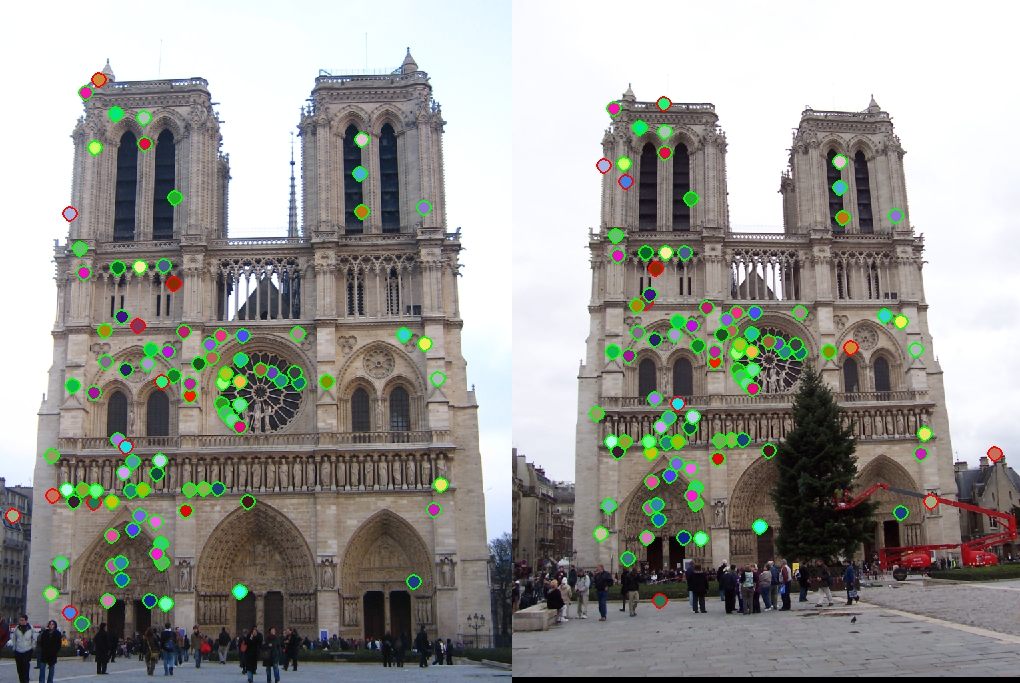
Example of SIFT feature matching.

Image Pyramid

The easiest way to deal with a scaling issue is to utilize image pyramids. We have multiple ways to building an image pyramid such as the Gaussian and Laplacian pyramids. Laplacian pyramids are commonly used when whe need to reconstruct an upsampled image from the pyramid. Since our evaluation function check the correctness simply by counting the pixels from the true location, the simplest downsample method is chosen. The code used to build the image pyramid is as follows:

% build an image pyramid
pyramid_scale = 0.75;
% set this to one to see the non-scale-invariant version
pyramid_num = 7; 
image_tmp = image1_bw;
image1_pyramids = cell(pyramid_num);
for i = 1:pyramid_num
    image1_pyramids{i} = image_tmp;
    image_tmp = imresize(image_tmp, pyramid_scale, 'bilinear');
end
image_tmp = image2_bw;
image2_pyramids = cell(pyramid_num);
for i = 1:pyramid_num
    image2_pyramids{i} = image_tmp;
    image_tmp = imresize(image_tmp, pyramid_scale, 'bilinear');
end

This image pyramid is used to find interest points, to obtain feature descriptors, and to compute feature matching; thus, the implementation is relatively robust to the scale variance. The results are discussed in the last section.

Corner Harris to find interest points

Typically, the SIFT features are computed around some interest points. When we use the dense SIFT, this is not always the case, but the implementation here uses the interest points extracted by the corner harris for the computation of the feature descriptors. The first step of the corner Harris is to compute the derivatives in both the x (width) and y (height) direction.

% compute derivatives
image = image_pyramids{pyramid};
g_deriv_x = fspecial('sobel');
g_deriv_y = g_deriv_x';

Ix = imfilter(image, g_deriv_x);
Iy = imfilter(image, g_deriv_y);
Ixx = Ix.^2;
Iyy = Iy.^2;
Ixy = Ix.*Iy;

After applying the Gaussian blurring, the cornerness function is computed as follows:

% compute cornerness
har = (Ixx .* Iyy - Ixy .^ 2 - alpha * ((Ixx + Iyy) .^ 2));

The locations that show the great cornerness are selected for the following procedures. The author uses three thresholds to select these interest points. The first threshold compares the point with the mean of the cornerness. This threshold is used in order to reduce the overall qualify of an image such as camera quality, brightness, exposure, and the weather. The original mean itself was too strong for this threshold, and then the mean is first scaled and used for the threshold. The second threshold checks if the location has the stronger cornerness than any of its neighbors. The third threshold directly evaluates the cornerness function.

reduce_mean = 0.1;
har = har .* (har > reduce_mean * (mean(mean(har))));
maxCheck = colfilt(har, [feature_width, feature_width], 'sliding', @max);
har = har .* ((har == maxCheck));
cornerThreshold = 1e-4;
[y, x, confidence] = find(har > cornerThreshold);

This operation is conducted with each image of the image pyramids, and all the corners that pass the above thresholds are stored with their scales.

ys(end+1:end+size(y, 1), 1) = y;
xs(end+1:end+size(x, 1), 1) = x;
confidences(end+1:end+size(confidence, 1), 1) = confidence;
scales(end+1:end+size(y, 1), 1) = scale;

Ys(end+1:end+size(ys, 1), 1) = ys;
Xs(end+1:end+size(xs, 1), 1) = xs;
Confidences(end+1:end+size(confidences, 1), 1) = confidences;
Scales(end+1:end+size(scales, 1)) = scales;
Pyramids(end+1:end+size(ys, 1), 1) = pyramid;

Feature descriptors

A scale invariant feature transform (SIFT) feature is computed around each of the interest points extracted by the above corner Harris method. The implementation allows a various widths of the features, but the bin size and the direction size are fixed to 4 x 4 and 8 directions, respectively. This means that each feature descriptor has 128 dimensions because each of the bin box stores 8 directions (4 x 4 x 8 = 128). What a feature descriptor stores is a histgram of the gradient orientation. For the corner location [x(i), y(i)], the correspoinding orientations can be computed in the following way:

region_size = feature_width / 2;
range_x = (x(i) - region_size):(x(i) + region_size - 1);
range_y = (y(i) - region_size):(y(i) + region_size - 1);
size_range_x = size(range_x, 2);
size_range_y = size(range_y, 2);
orientations_feature = zeros(size_range_x, size_range_y);
for j = 1:size_range_x
   for k = 1:size_range_y
       x_fd = Ix(range_y(j), range_x(k)); % x first derivative
       y_fd = Iy(range_y(j), range_x(k)); % y first derivative
       orientations_feature(j, k) = floor(atan2(y_fd, x_fd) / (pi / 4)) + 4;
   end
end

Also, the magnitude of the gradient is computed as follows:

mags = sqrt(abs(Ix).^2 + abs(Iy).^2);

The magnitude is downweighted by a Gaussian fall-off function beucase the influence of the gradient far from the interest point should be reduced. At this point, the magnitudes and orientations are stored in the box whose sizes are feature_width by featire_width. In order to compute the histgram in the 4 b 4 bins, the magnitudes and orientations are reshaped into 16 matrices, each of which corresponds to each of the bins.

% reshape 16 x 16 matrix into smaller submatrices
bin_num = 16;
bin_row = sqrt(bin_num);
bin_col = sqrt(bin_num);
bin_width = feature_width / bin_row;
bin_height = bin_width;
current_bin = 1;
orientations_r = zeros(bin_width, bin_height, bin_num);
mag_r = zeros(bin_width, bin_height, bin_num);
for j = 0:bin_row-1
    for k = 0:bin_col-1
        orientations_r(:, :, current_bin) = orientations_feature(j * bin_height + 1:(j+1)...
            * bin_height, k * bin_width + 1:(k+1) * bin_width); 
        mag_r(:, :, current_bin) = feature_mags(j * bin_height + 1:(j+1) * bin_height,...
            k * bin_width + 1:(k+1) * bin_width);
        current_bin = current_bin + 1;
    end
end

Finally, the normalized histgram makes one feature descriptor as follows.

% build histogram
% each feature has 128 dimensions and it stores the feature of the
% submatrix in the following order
% [topleft mat dir1, topleft mat dir2, dir3, ... topright mat dir1,
% dir 2, ... bottom right mat dir1, dir2, ... dir 8]
for current_bin = 1:bin_num
    for orientation = 1:8
        % note orientation is stored from 0 to 7
        [pos_x, pos_y] = find(orientations_r(:, :, current_bin) == (orientation - 1));
        num_found_orientation = size(pos_x);
        magnitude_sum = 0;
        for j = 1:num_found_orientation
            magnitude_sum = magnitude_sum + mag_r(pos_x(j), pos_y(j), current_bin);
        end
        features(i, 8 * (current_bin - 1) + orientation) = magnitude_sum;
    end
end
norm_feature = norm(features(i, :));
if(isfinite(norm_feature))
    features(i, :) = features(i, :)./norm_feature;
else
    fprintf('feature %d norm is not finite\n', i);
end

Matching points by Ratio Test

The matchmaker first compares the number of the feature descriptors from two images, and the smaller number of the two pairs are outputed from the matchmaker. The algorithm computes the Euclidean distance of the two features and searches the closest and the second closest feature for each. When the ratio of the first closest distance to the second surpasses the threshold, the feature pair is stored as a candidate for the evaluation. Also, the reciprocal of the ratio is used as a confidence; thus, the smaller the ratio, the better matching. This operation is done for all the features, and the features with the best 100 confidences are used for the evaluation. The codes used for the matching is shown below:

if(size(features1, 1) <= size(features2, 1))
    features_s = features1;
    features_l = features2;
else
    features_s = features2;
    features_l = features1;
end
BIG = 1e16;
num_features = size(features_s, 1);
used = zeros(size(features_l, 1));
matches = [];
confidences = [];
% Look at P.230 of the textbook
for i = 1:num_features
    firstClosestDis = BIG;
    secondClosestDis = BIG;
    firstClosest = -1;
    secondClosest = -1;
    current_feature = features_s(i, :);
    for j = 1:size(features_l, 1)
        dis = norm(current_feature - features_l(j, :));
        if(dis < firstClosestDis && used(j) == false)
            secondClosest = firstClosest;
            firstClosest = j;
            secondClosestDis = firstClosestDis;
            firstClosestDis = dis;
        end
    end
    nn = firstClosestDis / secondClosestDis;
    pairNow = [i firstClosest];
    nearestNeighborThreshold = 1.0;
    if(nn < nearestNeighborThreshold)
        confidences(end + 1, 1) = 1.0/nn;
        matches(end+1, :) = pairNow;
        used(firstClosest) = true;
    end
end
if(size(features1, 1) > size(features2, 1))
    matches = fliplr(matches);
end
[confidences, ind] = sort(confidences, 'descend');
matches = matches(ind, :);

Results

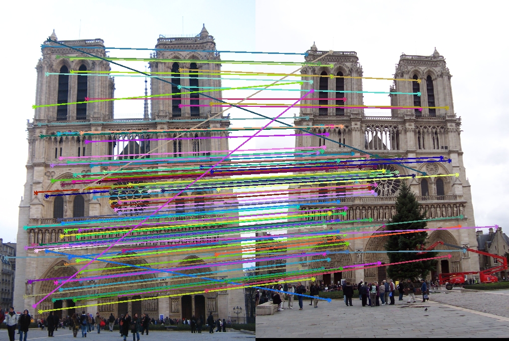
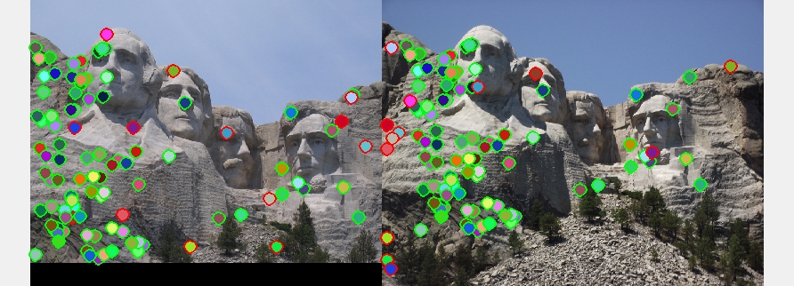
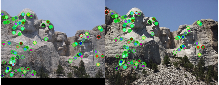
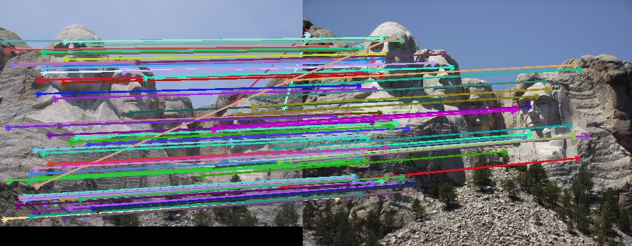
First, the figures below show the results with one layer of the image pyramids.

Correct (green) and incorrect (red) dots	Arrows connecting the matched pairs

Correct (green) and incorrect (red) dots	Arrows connecting the matched pairs

Correct (green) and incorrect (red) dots	Arrows connecting the matched pairs

Here, the only image used for the corner finding and feature descriptor is the original image scaled by the lines below:

scale_factor = 0.5; 
image1 = imresize(image1, scale_factor, 'bilinear');
image2 = imresize(image2, scale_factor, 'bilinear');

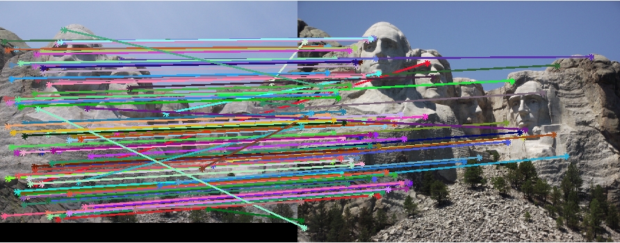
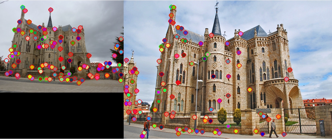
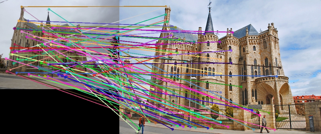
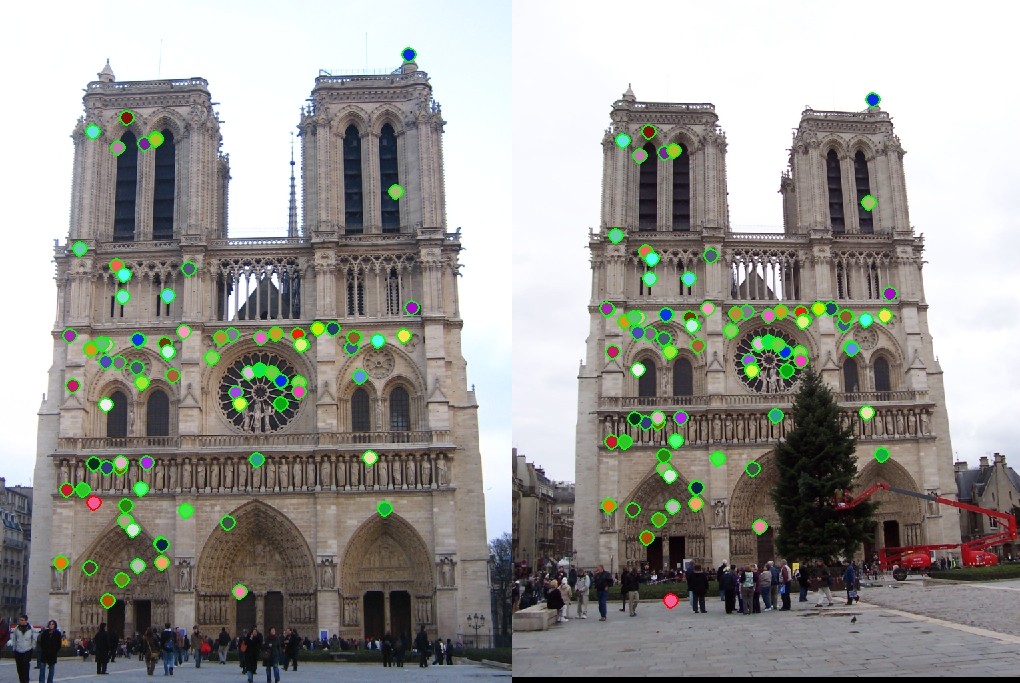
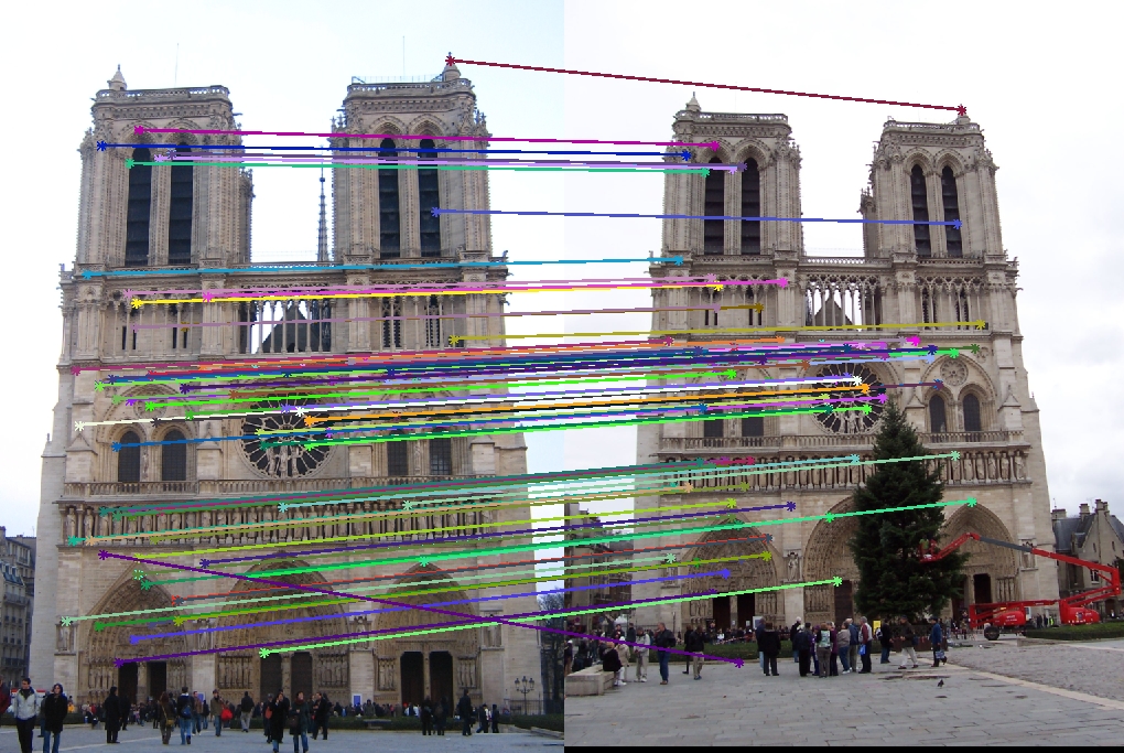
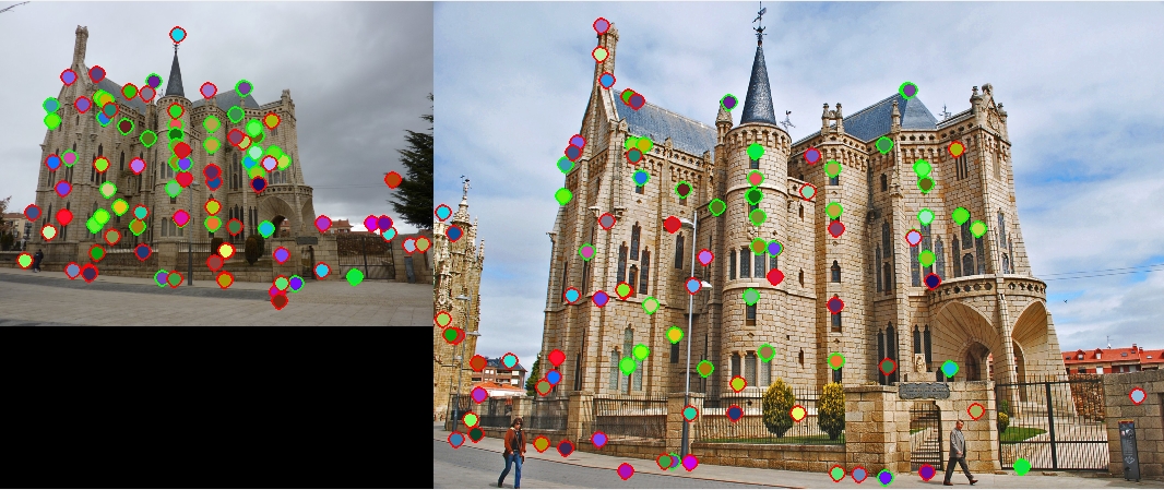
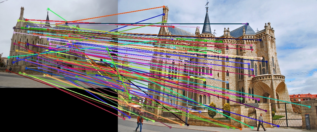
You can test the one-layer version simply by setting the parameter 'pyramid_num' in proj2.m to one. The results with the Nortre Dame and Mount Rushmore are already satisfactory, 90% and 87% correct. However, the results with the Episcopal Gaudi was very poor, and it showed only 8% correct. Apparently, the resolutions of the figures of the Episcopal Gaudi are a lot different between the pair. Since the same feature widths were used for both the images, a corner found at one image may not be found in the other. Also, the SIFT features are not perfectly scale invariant. These problems are mitigated by using the image pyramids. The figures below show the results with the image pyramids.

Correct (green) and incorrect (red) dots	Arrows connecting the matched pairs

Correct (green) and incorrect (red) dots	Arrows connecting the matched pairs

Correct (green) and incorrect (red) dots	Arrows connecting the matched pairs

The scales and the number of layers used for this demonstration are summarized below:

	Scale	Layers
Nortre Dame	0.85	5
Mount Rushmore	0.95	6
Episcopal Gaudi	0.75	6

Finding the right combination of the scale and the number of layers is a challenging task. The rule author created was if one image is a lot smaller than the other, the greater scale value is better, and vice versa. The number of the layers were increased until the success rate was satisfactory. All of the three pairs increased the success rate using the image pyramids. The results are summarized in the below table.

	Witout Image Pyramids	With Image Pyramids
Nortre Dame	90 %	99 %
Mount Rushmore	87 %	96 %
Episcopal Gaudi	8 %	44 %

Although the results of the Episcopal Gaudi are improved by far with the image pyramids, other methods than the image pyramids would be necessary to have a as good matching as the other pairs. More systematic tuning of the scaling factor and the number of layers may increase the success rate.