Vaibhav Dedhia

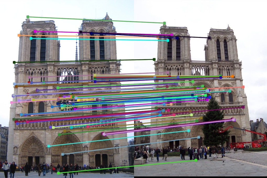
Example of Local feature matching.

Explanation:

1. Interest Point Detection/ Keypoint Detection

Interest point detection is a recent terminology in computer vision that refers to the detection of interest points for subsequent processing. An interest point is a point in the image which in general can be characterized as follows:

1. it has a clear, preferably mathematically well-founded, definition.
2. it has a well-defined position in image space.
3. the local image structure around the interest point is rich in terms of local information contents (e.g.: significant 2D texture).
4. it is stable under local and global perturbations in the image domain as illumination/brightness variations.
The Interest points can thus constitute of points on edges, corners, blobs, ridges etc. in an image.
2. Feature Description

Once the keypoints in the images are extracted, we would like to have some sort of matching between images of the same scene captured from different view points. However, these keypoints are not enough for direct comparision and hence some sort of more informative feature needs to be generated, using which tasks of comparision and matching can be simplified. To server this purpose, we extract the patch around the interest point and use the information from this patch to encode a descriptor that is suitable for discriminative matching. This encoded patch of feature is called feature descriptor.

3. Feature Matching

The feature descriptor we described in above step can directly be used for the local feature matching purpose. The euclidean distance the features are calculated and the two features which have minimum distance can be safely classified as matched features.

The implementation:

The project implementation has been done in Matlab. The keypoint detection is done using Harris detectors. It is rotation and translational invariance. It comprises of five steps: gradient computation, Gaussian smoothing, Harris measure computation, thresholding and non-maximum suppression. This algorithm is used to detect interest points of the images for which local feature matching is being done.

The feature descriptor has been achieved using SIFT. First a set of orientation histograms is created on 4x4 pixel neighborhoods around the interest point obtained from first step with 8 bins each. These histograms are computed from magnitude and orientation values of samples in a 16 x 16 region around the keypoint such that each histogram contains samples from a 4 x 4 subregion of the original neighborhood region. The descriptor then becomes a vector of all the values of these histograms. Since there are 4 x 4 = 16 histograms each with 8 bins the vector has 128 elements. This vector is then normalized to unit length in order to enhance invariance to affine changes in illumination. This process is used to compute features for all the interest points in first image and the process is repeated for the second image too.

Now, we can compare the SIFT features for both the images and have one to one correspondence. We have tried using the euclidean distance for feature matching. Also kd-tree algorithm was used which is discussed further in results.

Important Functions of Code

The Matlab code below shows the implementation of SIFT feature.

%SIFT code
    directions=8;
    [m,n]=size(image);
    count=1;
    xa=x;
    ya=y;
    for i=1:1:size(xa,1)
        x_count=1;
        for k=xa(i)-feature_width/2:1:xa(i)+(feature_width/2-1)
            y_count=1;
            for j=ya(i)-feature_width/2:1:ya(i)+(feature_width/2-1)
                 a(x_count,y_count) = image(j,k);
                y_count= y_count+1;
            end
            x_count=x_count+1;    
        end
        bin_angle = 360/ directions;
    
        [Gmag,Gdir] = imgradient(a);
        Gmag = Gmag(1:feature_width,:);
        Gdir = Gdir(1:feature_width,:);
        feature=[];
        for block_row=0:feature_width/4:feature_width-(feature_width/4)
            for block_col=0:feature_width/4:feature_width-(feature_width/4)
                dir_bin=zeros(1,directions);
                for u=1:1:feature_width/4
                    for v=1:1:feature_width/4
                        amag = Gmag(block_col+v,block_row+u);
                        adir = Gdir(block_col+v,block_row+u);
                        if(adir == 0)
                            adir=1;
                        elseif (adir<0)
                            adir = 360 - abs(adir);
                        end
                        rem = ceil(adir/bin_angle);
                        dir_bin(rem) = dir_bin(rem) + amag;

                    end    
                end
                for dir_loop = 1:1:directions
                    feature = [feature dir_bin(1,dir_loop)];  
                end 
            end    
        end

The Matlab code below shows the implementation of Harris Corner Detector.

%harris corner detector code
filter1 = fspecial('gaussian', [3 3], 0.5);
image = imfilter(image,filter1);
[Gx, Gy] = imgradientxy(image);
gx = Gx.*Gx;  %Ix2
gy = Gy.*Gy;  %Iy2
ggxy = gx.*gy;  %g(Ix.Iy)
new_image = gx.*gy - ggxy.*ggxy - 0.06*(gx + gy).*(gx + gy);

filter2 = fspecial('gaussian',[9 9], 0.5);
new_image = imfilter(new_image,filter2);

x=0;  y=0; co=1;
[row col] = size(image);

[ m n] =size(image);
%% local non max supression
for i=0:10:row-10
    for j=0:10:col-10
        max=0;max_pos_x=1;max_pos_y=1;
        for k=1:1:10
            for l=1:1:10
                if(new_image(i+k, j+l)>max)
                   new_image(max_pos_x, max_pos_y)=0;
                    max = new_image(i+k, j+l);
                    max_pos_x = i+k;
                    max_pos_y = j+k;
                else
                    new_image(i+k,j+l)=0;
                end
            end
        end
    end
end

%% interest point collection
        
        
for i=feature_width/2+1:1:row-(feature_width/2)
    for j=(feature_width/2)+1:1:col-(feature_width/2)
        if(new_image(i,j)>0.05)
           x(co,1)=j;
           y(co,1)=i;
           co = co+1;
        end
    end
end

Results

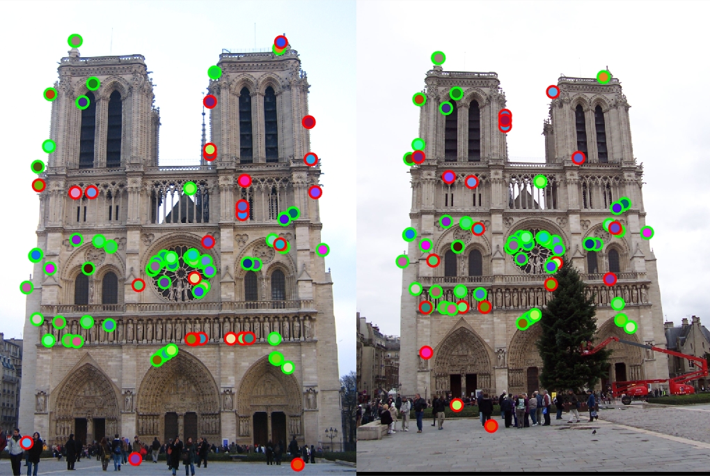
Local features.

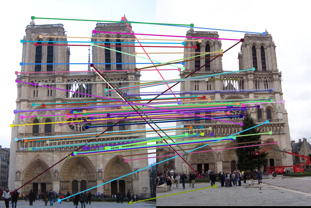
Local feature matching.

We have used harris corner detection for interest point detection. Non-local supression removes non-local maximum thus avoiding a dense number of interest points to be detected in a small region as it will redundantly increase the feature space. The threshold to classify points as corner points was experimentally set to 0.05. It returns a good number of features in images.

For feature extraction, we first used simple form of extraction: Normalized histogram patch. It basically extracts 4 X 4 neighbourhood patch around the interest points and creates a normalized histogram of the pixel values in this patch. This becomes the feature descriptor for that particular interest point and the procedure is repeated for all the interest points. It is also performed for both the second image. The accuracy obtained using normalized patch histogram is about 76% for 100 most confident searches. The accuracy obtained using SIFT was about 84% for 100 most confident features. Now, some parameters of SIFT were played around with, to test their effects on accuracy. In the standard SIFT feature implementation,we use the window-size to 16X16. We divide this patch into 4X4 pixel and obtain a 8-bin histogram for this. So, we have 128 dimensional vector for every feature. If instead of 16X16 window if we increase the window size to 32X32, the accuracy shoots to 93% for relatively low increase in computational time. In standard SIFT, we use 8 bin histogram. If instead of 8-bin, we use a higher bin histogram, the accuracy drops. For 10-bin histogram (i.e 10 directions), the accuracy drops to 82% (84% for 8 bin histogram) with 8 sec increase in time. If we try decreasing the bin number to 6, we see decrease in accuracy. So 8-bin histogram seems to be the ideal. There are various ways in which we can normalize histograms. I have tried using standard normalization technique, min-max normalization technique and the z-score. The z-score increase the accuracy to 86% while maintaining the time for execution.

For the feature matching, the standard euclidean technique for distance measurement takes 106 secs. To reduce the time taken, we tried implementing kd-tree. It is a space-partitioning data structure for organizing points in a k-dimensional space. Finding the nearest point is an O(log n) operation in the case of randomly distributed points. In high-dimensional spaces, the curse of dimensionality causes the algorithm to need to visit many more branches than in lower-dimensional spaces. In particular, when the number of points is only slightly higher than the number of dimensions, the algorithm is only slightly better than a linear search of all of the points. In our case, we create a kd map of features from second image and compare features from the first image with list of features from second image and match the closest pair of featurs. This gives accuracy of 86% with time taken being just 10.96 seconds.

The dimension reduction techniques like Principal component analysis can be used to create a vector space of lesser dimension, thus in turn reducing the computational time. PCA tries to summarize all the charachteristics of the vectors space with lesser number of dimensions. It tries to capture maximum variance in as little dimensions as possible. In our case, if we reduce the number of features from 128 to 32(i.e 4 times less), the accuracy still remains at 66% with a lesser computation time. In our case, the number of images, number of features is not that huge and the kd-tree does a fair job of reducing computational time. Thus, positive effect of PCA is not clearly evident in our case.

Applications

1. Image Stitching
2. 3d Scene reconstruction
3. Image Alignment
4. Object Recognition