Computer Vision Project

Project 2: Local Feature Matching

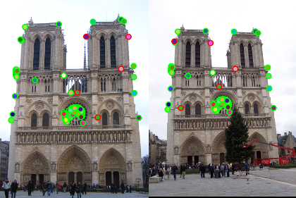
Final Notre Dame Result: 95% Accuracy on Top 100 Matches

Introduction

The goal of this assignment was to implement a local feature matching algorithm. These types of algorithms focus on identifying/matching common points between multiple views of the same scene. Generally, these types of algorithms are comprised of three steps (which together form a "pipeline"):

1. Identify interest points in the various views

2. Create local feature 'descriptions' around each interest point

3. Match features (and implicitly interest points) across views

My report proceeds as follows: First, I will describe the methodology I used to implement this pipeline. In my description, I will point out places where some bells & whistles work has been done. Second, I will show my baseline pipeline result with no bells and whistles. Third, I will show the marginal impact of including each bells and whistles item to the implementation. Fourth, and finally, I will show the results of my pipeline on additional image sets.

Methodology

Step 1: Identify interest points between views

Interest points are those that are repeatable and distinctive across views. While many interest point detectors exist, I implemented the Harris Corner Detector for this project. The Harris Corner Detector is built on the idea that ideal interest points are those for which a shift in any direction leads to a large change in intensity. A basic outline of how to determine Harris Corner points in an image can be described as follows:

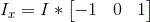
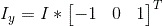
1. Compute the x and y gradients of the image -

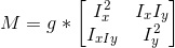
2. Use these derivatives to compute a second moment matrix M (where 'g' is some gaussian kernel of some choice dimension and stdev) -

3. Find the corner-ness score (R) for each pixel using the following equation (note, alpha can be between 0.04 and 0.06. I chose 0.04) -

3. Threshold the resultant corners - The corner-ness score given to each pixel by this process is >0 if the pixel is thought to be a corner, <0 if it is thought to be an edge, and 0 if it is thought to be a "flat" region. Thus, the first "thresholding" I do is to 0 out any score that is below 0.001.

4a. Non Maximal Suppression - Once I have all points that are corners, I'd like to minimize the chance that my corners are too "clustered" (i.e. they all lie on some part of the same corner). To do so, I implement two non-maximal suppression techniques. The first technique I use is to take a sliding 3x3 window across the image, and only keep the pixel with the maximum corner-ness score from each window.

4b. Further Bells & Whistles Work - The second technique I subsequently implement is Adaptive Non-Maximal Suppression (ANMS). This technique was listed on the bells and whistles suggestions, and effectively amounts to ranking corner points by their distance to the nearest corner point with a higher score. The top n (I use 1000) points with the greatest distance measure are kept for the remaining portions of the pipeline.

Step 2: Create local feature 'descriptions' around each interest point

1. First Pass Implementation - I followed the basic algorithm specified by SIFT:

a. Take a 16x16 window around each interest point

b. Split this 16x16 window into 16 4x4 subwindows

c. For each subwindow compute a histogram with 8 bins based on the possible orientations of the gradients of the pixels in that subwindow. Additionally, the values added into these bins are not simple "counts", but are rather gaussian down-weighted magnitudes. The 16x8 (128) bins that make up the total window are together the feature descriptor for the given interest point.

2. Bells & Whistles Work - Once I had the initial implementation completed, I decided to then try to tune the parameters related to feature creation (i.e. feature size, number of subwindows, number of histogram orientations). After much testing, I came to the conclusion that the only parameter tuning that seemed to really make a consistent difference was changing the feature size to 20 instead of 16. Any higher/lower from 20 and my accuracy on the top 100 decreased. Thus, I kept my feature size at 20 to create my final result.

3. Further Bells & Whistles Work - Once I had my first implementation completed, I then completed the Bells & Whistles option of implementing a flavor of the GLOH feature descriptor. This descriptor is created by doing the following:

1. Convert points around interest point to polar coordinates

2. Group these points into 17 sub-groups which are located at radius = 6, 11, 15 and angle = 0,45,90,...,360

3. Similar to SIFT, bin each sub-group into a 16 orientation histogram. The resulting 272 bins around each interest point make up the feature description.

Step 3: Match features (and implicitly interest points) across views

1. First Pass Implementation

- For each interest point feature descriptor from the first image, take the euclidean distance to every feature descriptor from the second image:

- Find the Nearest-Neighbor Distance Ratio (nndr). If this ratio is some number less than 1 (i.e. the first match is closer than the second - I chose 0.88 as my threshold), keep the two points as a potential match, and mark the 'confidence' of the match

- Take the highest n confidence matches and evaluate them

2. Potential Bells & Whistles Work - At the end of Szeliski 4.1.3, he mentions using RANSAC to try to estimate a homography between the two views using the high confidence points from the NNDR step. While it wasn't explicitly listed as a Bells & Whistles item, I decided to implement this technique out of curiosity. In short the idea is that you want to try to estimate the the mathematical mapping between the two views (the homography, h):

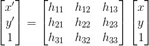
You need to use four points at a time to estimate the homography. Once the homography is estimated, it can then be used to predict locations of second view points based on first view points. If you set a threshold on what an acceptable distance between the estimated second view points and the actual second view points should be, you can then loop over the homography estimation and prediction process until you get a homography that yields that highest number of acceptable mappings.

This is largely what I do in my implementation - After I compute the NNDR and corresponding confidences, I use the 100 most confident matches to run through the homography estimation/prediction 1000 times (each time randomly sampling 4 of the 100 most confident matches). At the end of this process, I'm left with a matches vector that is not only based on feature descriptions, but also on the underlying geometry between the two scenes.

Baseline Pipeline Result

This baseline pipeline (no Feature Size Change/ANMS/GLOH/RANSAC), produced 77% accuracy on the top 100 results.

Marginal Effect of Feature Size Change/ANMS/GLOH/RANSAC Inclusion

In order to see how much each Bells & Whistles addition helped, I think it is valuable to see the accuracy changes based on the inclusion of each feature. Rather than iteratively add on each of these features to the baseline result presented above, I think it's more instructive to only try one of these features at a time. This way I can avoid dealing with the impact of the order in which I added things to the baseline implementation (i.e. potential cross terms).

Description Image Result Comments

Baseline Pipeline + Feature Size Change
Accuracy on top 100 matches goes up from 77% (baseline) to 84%

Baseline Pipeline + ANMS
Accuracy on top 100 matches goes up from 77% (baseline) to 82%

Baseline Pipeline Using GLOH Descriptor
Accuracy on top 100 matches goes up from 77% (baseline) to 84%

Baseline Pipeline + RANSAC
Accuracy on top 100 matches goes up from 77% (baseline) to 79%

Baseline Pipeline + Feature Size Change + ANMS + GLOH + RANSAC
Accuracy on top 100 matches goes up from 77% (baseline) to 89%. As expected, we get a big pick-up in performance by piling all the features on simultaneously.

Baseline Pipeline + Feature Size Change + ANMS + RANSAC (Final Implementation)
Accuracy on top 100 matches goes up from 77% (baseline) to 95%. Interestingly, by not using the GLOH descriptor (and instead by using the original SIFT descriptor), we get a much higher accuracy. I'm not convinced that this is a particularly robust result across all images. For the purposes of this assignment, however, this is my final implementation/result.

Description	Image Result	Comments
Baseline Pipeline + Feature Size Change		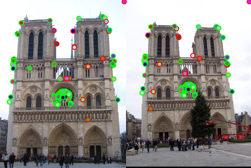Accuracy on top 100 matches goes up from 77% (baseline) to 84%
Baseline Pipeline + ANMS		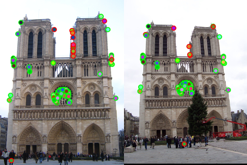Accuracy on top 100 matches goes up from 77% (baseline) to 82%
Baseline Pipeline Using GLOH Descriptor		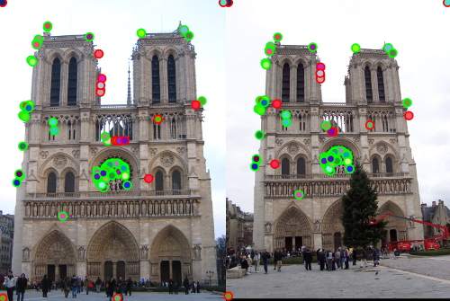Accuracy on top 100 matches goes up from 77% (baseline) to 84%
Baseline Pipeline + RANSAC		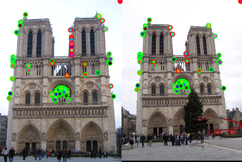Accuracy on top 100 matches goes up from 77% (baseline) to 79%
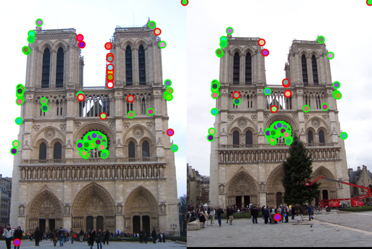
Baseline Pipeline + Feature Size Change + ANMS + GLOH + RANSAC		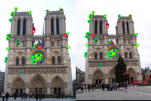Accuracy on top 100 matches goes up from 77% (baseline) to 89%. As expected, we get a big pick-up in performance by piling all the features on simultaneously.
Baseline Pipeline + Feature Size Change + ANMS + RANSAC (Final Implementation)		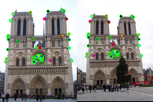Accuracy on top 100 matches goes up from 77% (baseline) to 95%. Interestingly, by not using the GLOH descriptor (and instead by using the original SIFT descriptor), we get a much higher accuracy. I'm not convinced that this is a particularly robust result across all images. For the purposes of this assignment, however, this is my final implementation/result.

Final Implementation Applied to Additional Test Sets

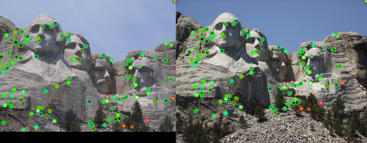
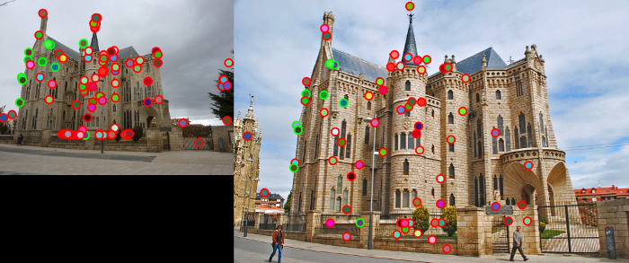
Mount Rushmore: 93% Accuracy on Top 100 Matches