Project 2: Local Feature Matching
The goal of this project is to implement a local feature matching algorithm. The pipeline adopted is a simplified version of the famous SIFT pipeline. The matching pipeline is intended to work for instance-level matching - multiple views of the same physical scene. In order to detect features and also discuss how feature correspondences can be established across different images, three steps are involved:
- Interest point Detection
- Local feature Description
- Feature Matching
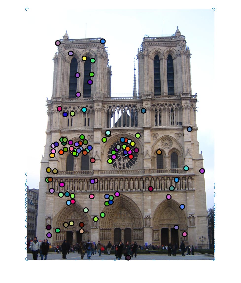
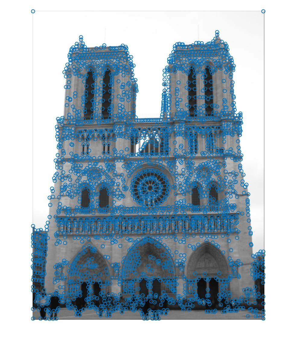
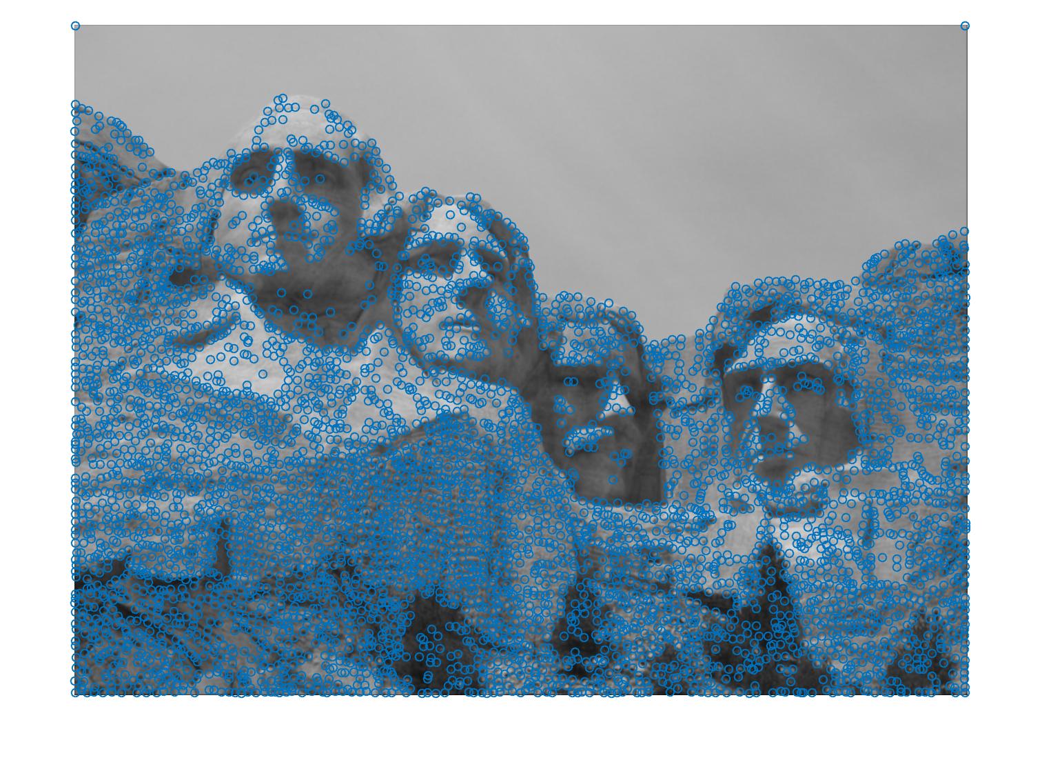
1. Detection : Identifying the interest points
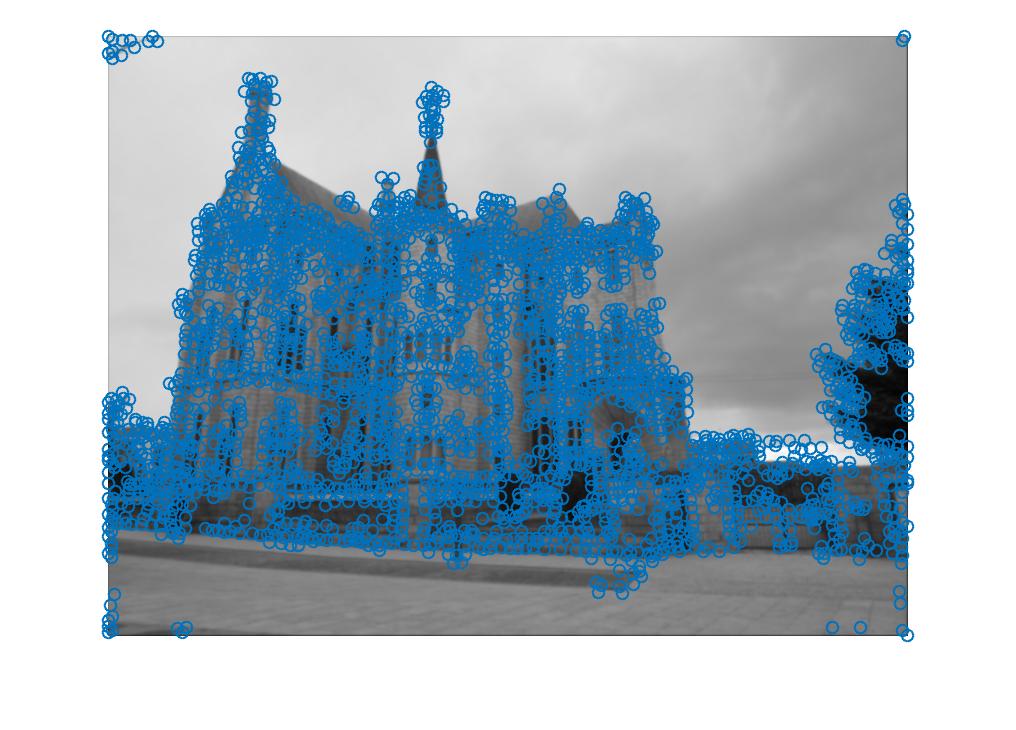
Interest points are detected using the Harris corner detector. The horizontal and vertical derivatives of the image are obtained and the images corresponding to the outer product of these gradients are computed. The image is first filtered using a Gaussian filter to remove noise. A scalar interest measure R is computed. Local maxima above a certain threshold is found out and they are reported as detected feature locations. After applying gradients, the points extracted from the gradient value are still quite blurred. But, there should only be one accurate response to the edge. Thus non-maximum suppression is incorporated to help suppress all the gradient values to 0 except the local maxima. The threshold value is changed according to different images.
2.Descriptor : Extract vector feature descriptor around each interest point
A SIFT like local feature is implemented. At each detected key point, the estimate of average gradient is calculated using region around the key point (a 16x16 region here). A weighted gradient orientation histogram is then computed in each sub region. This project uses 16 × 16 patches and for each 4 × 4 array, an 8 eight-bin histogram is computed. This results in a feature of 128 dimensions at each interest point.
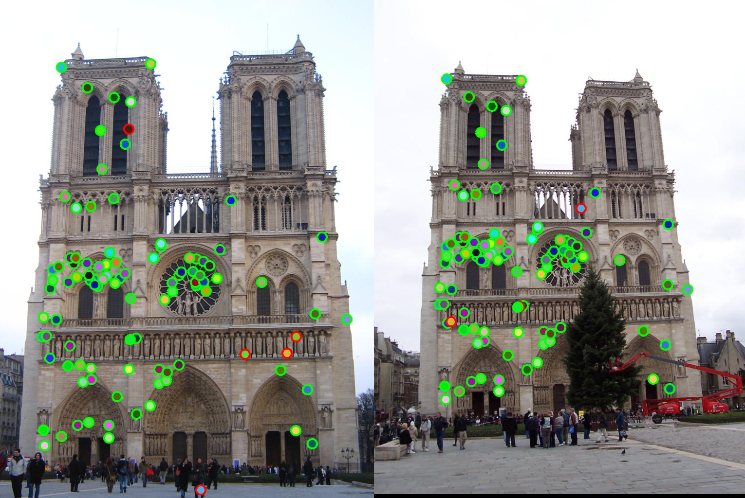
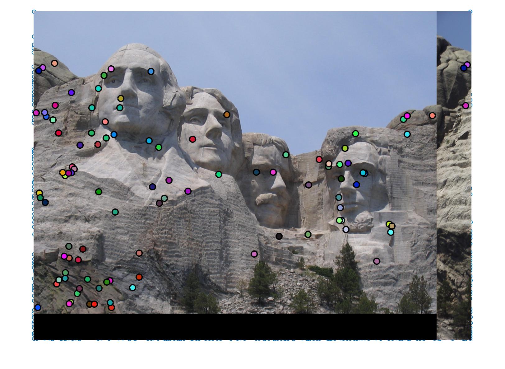
3.Matching : Determine correspondence between descriptors in two views
Local features are mapped using the "ratio test" or "nearest neighbor distance ratio test". The features computed for both the images in the previous functions are compared. A nearest neighbour distance is computed as the ratio of distance of first nearest neighbour and second nearest neighbour for a particular feature. The rationale behind this is that the first neighbour should be very similar and the second neighbour further away to indicate a single good match between feature points. Thus, the NNDR ratio should be as low as possible. The features that have this confidence value lesser than a predefined threshold are matched.
Tuning parameters
There are a number of parameters that I experimented with, The Filter - Initially used Sobel filter to get the interest points, then tried Gaussian filter followed by image gradients. The variance and size of the Gaussian filter was crucial and for each of the stages of filtering in the algorithm, these had to be accurately tuned.Threshold Value(R)- The threshold value affects both the quality and number of interest points obtained. For the Gaudi pair, the number of interest points obtained was fairly low and thus, for this pair I had to reduce the R threshold to 0.0001 from 0.01.
Alpha value - I used an alpha value of 0.01 rather than the suggest 0.04 and I found that it gave me better accuracy on the Notre Dame and Rushmore pairs.
Threshold value for NNDR - I rejected all matches that had an NNDR higher than 0.84 as being weak matches.
Initially I was getting an accuracy of 82% with the suggested baseline implementation and the Sobel filter for image gradients in the get interest points function. After tuning these parameters, I was able to achieve an accuracy of 98% on the Notre Dame pair.
Results
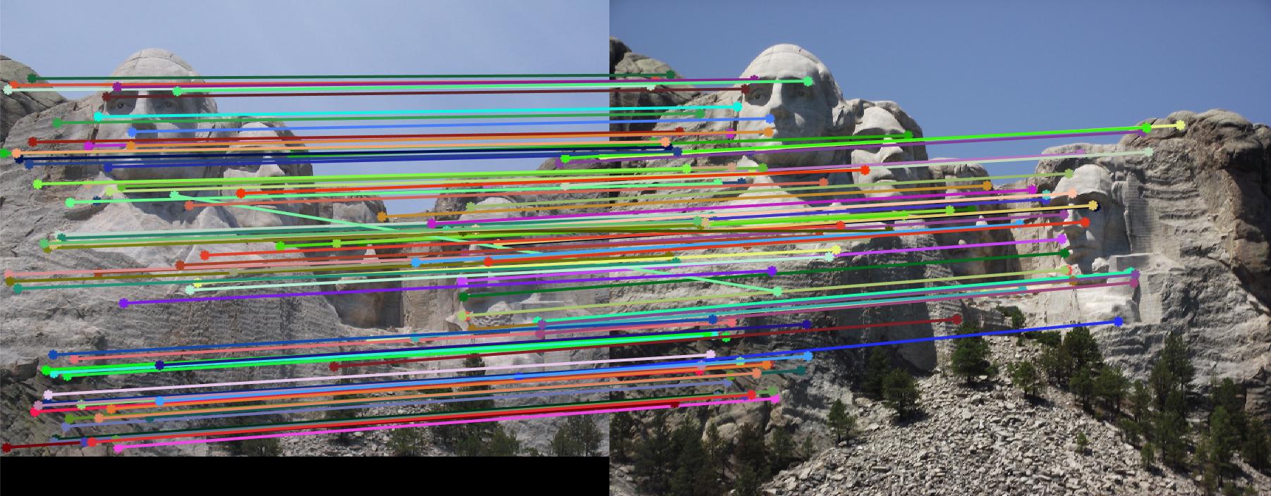
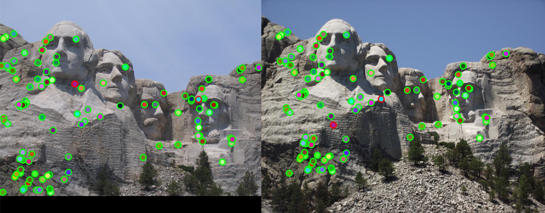
Mount Rushmore: 98% accuracy of the top 100 matches
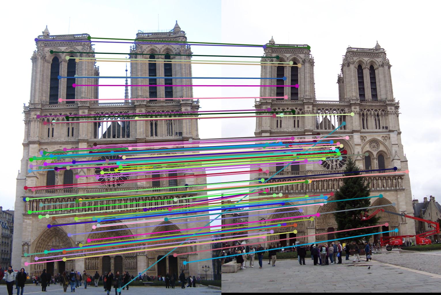
Notre Dame: 95% accuracy of the top 100 matches
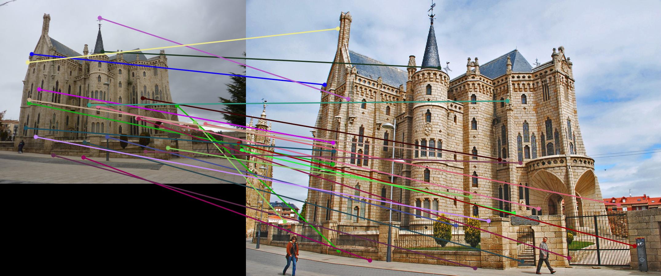
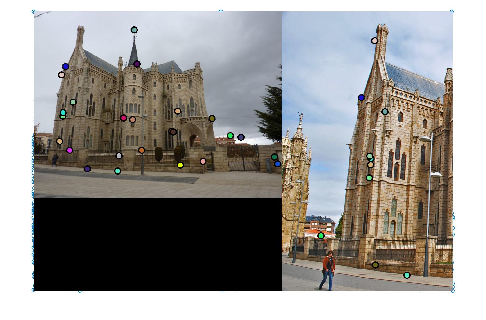
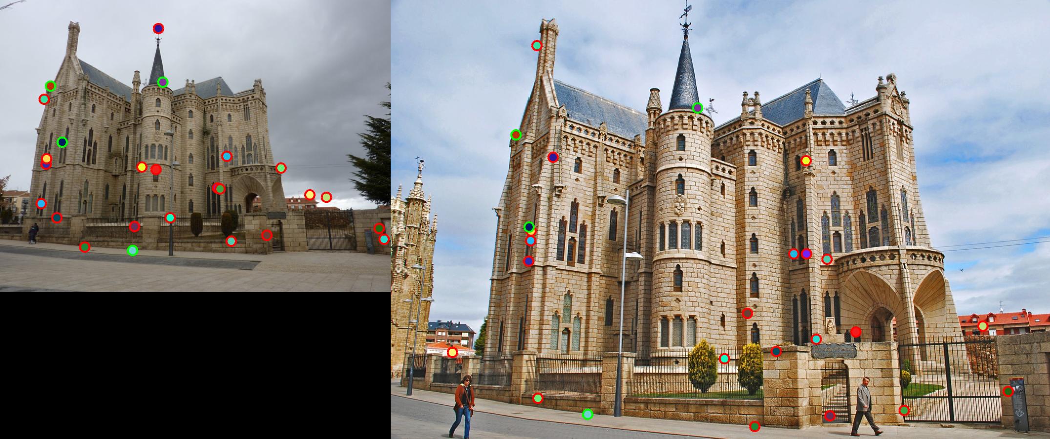
Gaudi: For this image I was only able to get 13 matches that satisfied the match confidence thresholding criteria. Of these, I obtained 3 good matches, giving a 23% accuracy.
Results of interest point detection and feature matching
|
|
|