Project 2: Local Feature Matching
The goal of this assignment is to create a local feature matching algorithm using a simplified version of the famous SIFT pipeline. The matching pipeline is intended to work for instance-level matching -- multiple views of the same physical scene.
My algorithm implementation
Interest Point Detection
In this part, based on the Harris corner detetor algorithm, i following the instruction on "Brown, M., Szeliski, R., and Winder, S. (2005). Multi-image matching using multi-scale oriented patches. In IEEE Computer Society Conference on Computer Vision and Pattern Recognition (CVPR2005), pp. 510-517, San Diego, CA." to impliment keypoints at multiple scales, For each interest point, i also compute an orientation, and in addition, i adopt adaptive non-maximal suppression to filter the amount of interest points.
The interest points we use are multi-scale Harris corners. For each input image image I(x,y) we form a Gaussian image pyramid Pl(x,y) using subsampling rate s = 2 and pyramid smoothing width sigma = 1.0. Interest points are extracted from each level of the pyramid.
The Harris matrix at level l and position(x,y) is smoothed outer product of the gradients

we set the intergration scal sigma = 1.5 and the derivative scale sigma = 1.0. To find interest points. The confident of the interesting point is given as the following:
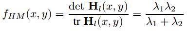
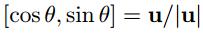
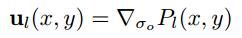
Interest points are located where the corner strength fHM (x, y) is a local maximum in neighbourhood, the orientation is given by:
The code for this aglrithm is presented as the following.
function [muti_x, muti_y, muti_confidence, scale, muti_orientation] = get_interest_points(image, feature_width)
muti_x =[];
muti_y = [];
scale = [];
muti_confidence = [];
muti_orientation = [];
im = image;
%scales =  2.^(1:-.5:-3); %detect interest point in mutiscale
scales =  2.^(0);

for si = 1:numel(scales)
    image = imresize(im, scales(si)) ;

    filterdel = fspecial('sobel');
    filterdel = rot90(filterdel);

    filter_orientation = [-4.5, 0, 4.5];

    I_x = imfilter(image, filterdel);
    I_y = imfilter(image, filterdel');
    I_x_2 = imfilter(I_x, filterdel);
    I_y_2 = imfilter(I_y, filterdel');
    I_x_I_y = imfilter(I_x, filterdel');

    I_orie_x = imfilter(image, filter_orientation);
    I_orie_y = imfilter(image, filter_orientation);

    gaussian2 = fspecial('gaussian', [25,25],1.5);

    A = imfilter(I_x_2, gaussian2);
    C = imfilter(I_y_2, gaussian2);
    B = imfilter(I_x_I_y, gaussian2);

    M_det = A.*C-B.^2;
    M_tr = A+C;
    R = M_det-0.06*M_tr.^2;

    % we don't need the interest point in the edge of the image, which
    % will influence the computation of representation

    feature_width = feature_width*2;
    R(1 : feature_width, :) = 0;
    R(end - feature_width : end, :) = 0;
    R(:, 1 : feature_width) = 0;
    R(:, end - feature_width : end) = 0;

    conn_comp = bwconncomp(im2bw(R, graythresh(R)));
    x = zeros(conn_comp.NumObjects,1);
    y = zeros(conn_comp.NumObjects,1);
    confidence = zeros(conn_comp.NumObjects,1);
    orientation = cell(conn_comp.NumObjects,1);

    %parfor i=1:conn_comp.NumObjects  %uncomment to accelerate the code
    for i=1:conn_comp.NumObjects
        region = conn_comp.PixelIdxList{i};
        [confidence(i), index] = max(R(region));
        [y(i), x(i)] = ind2sub(size(R), region(index));

        % orientation of the interest points
        P = [I_orie_x(x(i)), I_orie_y(y(i))];
        orientation{i} = P/norm(P);
    end
    [x, y] = ANMS (y, x, R);
    muti_x = [muti_x;x];
    muti_y = [muti_y;y];
    scale = [scale;scales(si)*ones(size(x))];
    muti_confidence = [muti_confidence; confidence];
    muti_orientation = [muti_orientation; orientation];
end
end
Adaptive Non-Maximal Suppression
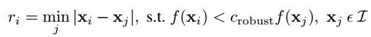
Since the computational cost of matching is superlinear in the number of interest points, it is desirable to restrict the maximum number of interest points extracted from each image. At the same time, it is important that interest points are spatially well distributed over the image. Interest points are suppressed based on the corner strength fHM , and only those that are a maximum in a neighbourhood of radius r pixels are retained.In practice we robustify the non-maximal suppression by requiring that a neighbour has a sufficiently larger strength. Thus the minimum suppression radius ri is given by
function [Rx, Ry] = ANMS (y, x, R)
%find the maxizm
max = -inf;
for i = 1:size(x)
    if(R(y(i),x(i))>max)
        max = R(y(i), x(i));
    end
end
Rmax = max*0.9;

%calculate the dist
Rdis = ones(size(x))*inf;
for i = 1:size(x)
    if(R(y(i), x(i))>=Rmax)
        Rdis(i) = inf;
    else
        for j=1:size(x)
            if (j~=i && R(y(j),x(j))*0.9>R(y(i),x(i)))
                dis = norm([y(j)-y(i),x(j)-x(i)]);
                if(dis < Rdis(i))
                    Rdis(i) = dis;
                end
            end
        end
    end
end
[dist, index] = sort(Rdis);

%select last 2000
Rx = x(index(end-2000:end));
Ry = y(index(end-2000:end));
end
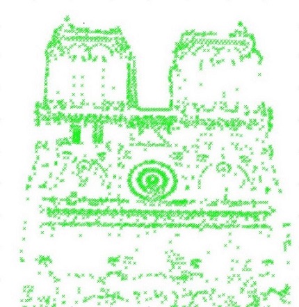
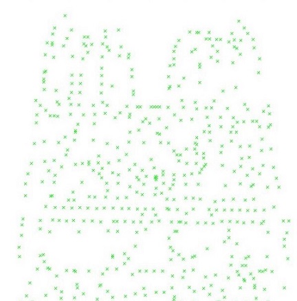
after ANMS with 500 points
Feature Descriptors
I implemented the baseline SIFT-like feature descriptors, the basic approach is as the following:
- Obtain a 16 by 16 window matrix around each keypoint.
- Compute the gradient magnitude and direction for each window.
- Weight the magnitudes according to their distance from the center pixel by using a gaussian filter.
- Break the window up into 16 cells of size 4 x 4.
- Form a histogram for each cell, dividing the gradients into 8 buckets, each covering 45 degrees.
- Sum the weighted magnitudes of the gradients in each bucket.
- Append each cell's histogram to form the 1 x 128 feature descriptor vector.
function [features] = get_features(image, x, y, feature_width)

angle_bins = -180:45:180;
features = zeros(length(x), 128);
half_width = int32(feature_width/2);
quarter_width = int32(feature_width/4);
% for each keypoint
for i = 1 : length(x)
    patch = image(y(i) - half_width : y(i) + half_width - 1, ...
        x(i) - half_width : x(i) + half_width - 1);
    [gmag, gdir] = imgradient(patch);
    gmag_weighted = imfilter(gmag, fspecial('gaussian', 16, sqrt(feature_width/2)));
    gmag_cols = im2col(gmag_weighted, [quarter_width, quarter_width], 'distinct');
    gdir_cols = im2col(gdir, [quarter_width, quarter_width], 'distinct');
    % for each cell in 4x4 array
    descriptor = zeros(1, 128);
    for j = 1 : size(gdir_cols, 1)
        col = gdir_cols(:, j);
        [~, inds] = histc(col, angle_bins);
        buckets = zeros(1, 8);
        for k = 1 : length(inds)
            buckets(inds(k)) = buckets(inds(k)) + gmag_cols(k, j);
        end
        descriptor(j*8-7 : j*8) = buckets;
    end
    %l_2 Normalization
    descriptor = descriptor / norm(descriptor);
    %power normalization
    descriptor = descriptor.^0.6;
    features(i, :) = descriptor;
end
end
I also impliment the Histogram of Oriented Gradients (HOG) descriptor as the following, but the performance is not satisfy since the HOG is not a robust descrptor in image matching:
function HOGFeature = get_features_hog( Img , x, y, feature_width)
cell_size=8;
nblock=2;
angle=180;%360
bin_num=9;
if size(Img,3) == 3
    G = rgb2gray(Img);
else
    G = Img;
end
hx = [-1,0,1];
hy = -hx';
grad_x = imfilter(double(G),hx);
grad_y = imfilter(double(G),hy);
% mod
grad_mag=sqrt(grad_x.^2+grad_y.^2);
% orientaion
index= grad_x==0;
grad_x(index)=1e-5;
YX=grad_y./grad_x;
if angle==180
    grad_angle= ((atan(YX)+(pi/2))*180)./pi;
elseif angle==360
    grad_angle= ((atan2(grad_y,grad_x)+pi).*180)./pi;
end
% orient bin
bin_angle=angle/bin_num;
grad_orient=ceil(grad_angle./bin_angle);
% num of block
block_size=cell_size*nblock;
point_num = size(x,1);
feat_dim=bin_num*nblock^2;
HOGFeature=zeros(feat_dim, point_num);
for k=1:point_num
    x_off = x(k)-int32(block_size/2);   %(j-1)*skip_step+1;
    y_off = y(k)-int32(block_size/2);   %(k-1)*skip_step+1;
    % magnitude and orientation of block
    b_mag=grad_mag(y_off:y_off+block_size-1,x_off:x_off+block_size-1);
    b_orient=grad_orient(y_off:y_off+block_size-1,x_off:x_off+block_size-1);
    % hog of block
    currFeat = BinHOGFeature(b_mag, b_orient, cell_size,nblock, bin_num, false);
    HOGFeature(:, k) = currFeat;
end
end

function blockfeat = BinHOGFeature( b_mag, b_orient, cell_size, nblock, bin_num, weight_gaussian)
blockfeat=zeros(bin_num*nblock^2,1);
% gaussian weight
gaussian_weight=fspecial('gaussian',cell_size*nblock,0.5*cell_size*nblock);
for n=1:nblock
    for m=1:nblock
        % cell
        x_off = (m-1)*cell_size+1;
        y_off = (n-1)*cell_size+1;
        % cell magnitute and orientation
        c_mag=b_mag(y_off:y_off+cell_size-1,x_off:x_off+cell_size-1);
        c_orient=b_orient(y_off:y_off+cell_size-1,x_off:x_off+cell_size-1);
        % cell'hog
        c_feat=zeros(bin_num,1);
        for i=1:bin_num
            if weight_gaussian==false
                c_feat(i)=sum(c_mag(c_orient==i));
            else
                c_feat(i)=sum(c_mag(c_orient==i).*gaussian_weight(c_orient==i));
            end
        end
        % combine
        count=(n-1)*nblock+m;
        blockfeat((count-1)*bin_num+1:count*bin_num,1)=c_feat;
    end
end
%L2-norm
sump=sum(blockfeat.^2);
blockfeat = blockfeat./sqrt(sump+eps^2);
end
Feature Matching
In the feature_matching section i use PCA to decrease the dimention of the Sift decriptor due to limited feature, the base of PCA is obained by compute all the feature to be matched(actually with more training datas, we can obtain more robust base of PCA). And also i use kd-tree in the VL_feat libary to accelarate matching.
function [matches, confidences] = match_features(features1, features2)

% This function does not need to be symmetric (e.g. it can produce
% different numbers of matches depending on the order of the arguments).

% To start with, simply implement the "ratio test", equation 4.18 in
% section 4.1.3 of Szeliski. For extra credit you can implement various
% forms of spatial verification of matches.

% Placeholder that you can delete. Random matches and confidences

num_f1 = size(features1,1);
num_f2 = size(features2,1);
eucl_dis = zeros(num_f2, num_f1);
confidences = zeros(num_f1,1);
matches = zeros(num_f1,2);

numPcaDimensions = 100;
descrs = [features1;features2]';
encoder.projectionCenter = mean(descrs,2) ;
x = bsxfun(@minus, descrs, encoder.projectionCenter) ;
X = x*x' / size(x,2) ;
[V,D] = eig(X) ;
d = diag(D) ;
[d,perm] = sort(d,'descend') ;
%d = d + opts.whiteningRegul * max(d) ;
m = min(numPcaDimensions, size(descrs,1)) ;
V = V(:,perm) ;
%whitening
%encoder.projection = diag(1./sqrt(d(1:m))) * V(:,1:m)' ;
encoder.projection = V(:,1:m)' ;
features1 = (encoder.projection * bsxfun(@minus, features1', encoder.projectionCenter))' ;
features2 = (encoder.projection * bsxfun(@minus, features2', encoder.projectionCenter))' ;

  run(fullfile(fileparts(which(mfilename)), ...
               'vlfeat-0.9.20', 'toolbox', 'vl_setup.m')) ;

% for i = 1:num_f1
%     for j=1:num_f2
%        eucl_dis(j,i) = norm(features1(i,:) - features2(j,:));
%     end
% end
% [sorted, index] = sort(eucl_dis);

kdtree = vl_kdtreebuild(features2', 'numTrees', 1) ;
 [words,distances] = vl_kdtreequery(kdtree, features2', ...
                                     features1', ...
                                     'NUMNEIGHBORS', 2);%,...
                                     %'MaxComparisons', 1) ;


for i=1:num_f1
    NNDR = distances(1,i)/distances(2,i);
    %NNDR2 = sorted(1,i)/sorted(2,i);
    if NNDR < 0.99%0.7%0.65
        %matches(i,:) = [i, index(1,i)];
        matches(i,:) = [i, words(1,i)];
        confidences(i) = 1-NNDR;
    end
end

matches = matches(find(confidences>0),:);
confidences = confidences(find(confidences>0));

% Sort the matches so that the most confident onces are at the top of the
% list. You should probably not delete this, so that the evaluation
% functions can be run on the top matches easily.
[confidences, ind] = sort(confidences, 'descend');
matches = matches(ind,:);
Result
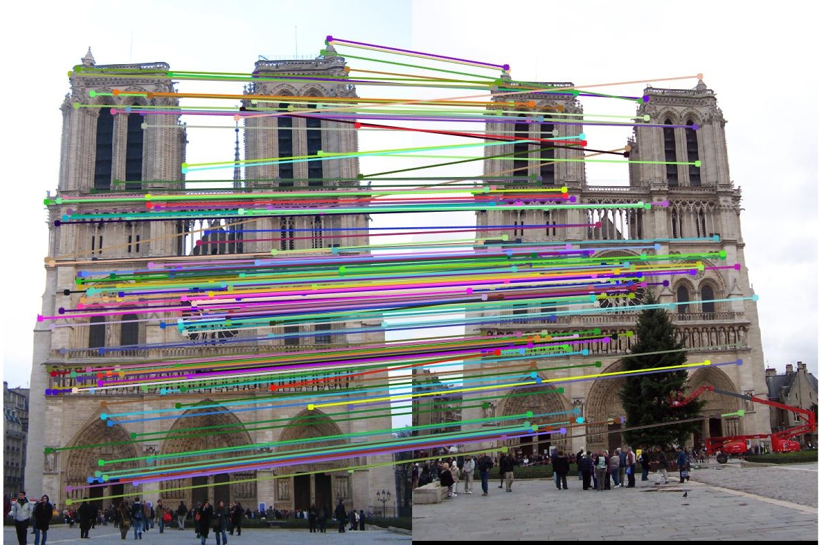
For the Notre Dame test images, 167 total good matches, 29 total bad matches. 0.85% accuracy