William Su

Example of a right floating element.

Finding the interest points

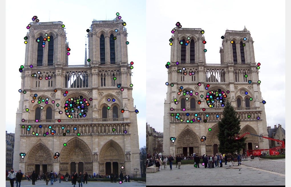
Interest points in the images were found by using the Harris Corner Detection algorithm. The algorithm uses a sobel filter in order to find interest points. I filtered the image and the tranpose of the image against the sobel filter in order to get the corresponding x and y matrices to input into the formula below:

Ix and Iy represents filtered image and image transpose matrixes. Once the matrix components were obtained, I ran each matrix component against a gaussian filter, which is represented as w in the formula. Once A was obtained, I used the follow formula to compute a matrix of interest points:

The outputed matrix was then used to separate the pixels in order to output an x and y coordinate arrays of interest points.

Example of Partial Harris Detection Code

hmat is the matrix that contains all the potential interest points

	binary = imbinarize(hmat);
	components = bwconncomp(binary);
    
    
    numOfComponents = components.NumObjects;
	x = zeros(numOfComponents, 1);
	y = zeros(numOfComponents, 1);
    
	for i = 1 : numOfComponents
	    pixelList = components.PixelIdxList{i};
        componentInHmat = hmat(pixelList);
        
        %finds max pixel index in hmat
	    [maxVal, ind] = max(componentInHmat);
        hsize = size(hmat);
        
        values = pixelList(ind);
	    [y(i), x(i)] = ind2sub(hsize, values);
        
    end

BWCONNCOMP was used in order to find the component regions in the image. This basically just groups pixels together that have similar aspects. From there on, the components were sorted out and the pixels were added to the x and y array.

Getting the features

Features were obtained using SIFT-feature descriptors. The approach to this algorithm is quite lengthy. First a space needs to be create around each interest point which is a 16x16 matrix. This can be seen with the code below. feature_width is 16 in this case.

	ylower = y(ind) - feature_width/2;
	yupper = y(ind) + feature_width/2 - 1;
	xlower = x(ind) - feature_width/2;
	xupper = x(ind) + feature_width/2 - 1;
	space = image(ylower : yupper, xlower : xupper);

For each space matrix that is created, the gradient magnitude and direction needs to be calculated, and the magnitude is then weighted using a gaussian filter. Afterwards, the matrix space is then broken up into 4x4 cells, and a histogram for each cell is formed. The gradients will be divided into 8 buckets of degrees starting from 0 and ending at 360 with increments of 45. This is because there are 8 parts to a feature: 4 diagonals, 2 horizonal, 2 vertical. The gradients from each part will then be accumulated, which is represented as a histogram. This is then appended to the features matrix, which is then normalized in order to achieve more accurate results. The code for this the histograms can be viewed below:

cell_size = feature_width/4;
        
%this breaks the feature into 4x4 cells
direction_columns = im2col(unit_direction, [cell_size, cell_size], 'distinct');

gauss_mag_columns = im2col(magnitude_with_gauss, [cell_size, cell_size], 'distinct');

des = zeros(1,128);
rows = size(direction_columns, 1);
for r = 1:rows
    
    %the 8 directions in the grid
    direction_col = direction_columns(:, r);
    spikes_range = -180:45:180;
    
    bars = zeros(1, 8);
    [bincounts, indices] = histc(direction_col, spikes_range);
    for i = 1:length(indices)
        current_mag = gauss_mag_columns(i, r);
        %accumulate the magnitudes into corresponding buckets
        bars(indices(i)) = bars(indices(i)) + current_mag;
    end
    
    %add the histogram to the descriptors of the feature
    des(1, ((r - 1) * 8 + 1) : ((r - 1) * 8 + 8)) = bars;
end

features(ind,:) = des;

Matching the features

This part is much simpler to implement than the previous two parts. The euclidian distance for the two sets of features were calculated. These distances were then sorted in order to obtain the shortest distances, and if pass a certain threshold, then some of the points were filtered out. The features that did pass the test were able to successfully be returned into the matches matrix.

	num_features = min(size(features1, 1), size(features2,1));

	threshold = 0.80;
	distances = pdist2(features1, features2, 'euclidean');


	[sorted, indices] = sort(distances, 2);

	%get the smallest dists
	column1 = sorted(:, 1);
	column2 = sorted(:, 2);
	inverse_confidences = column1 ./ column2;
	lessMatrix = inverse_confidences < threshold;
	confidences = 1./inverse_confidences(lessMatrix);


	matSize = size(confidences, 1);
	matches = zeros(matSize, 2);
	matches(:,1) = find(inverse_confidences < threshold);
	matches(:,2) = indices(inverse_confidences < threshold, 1);

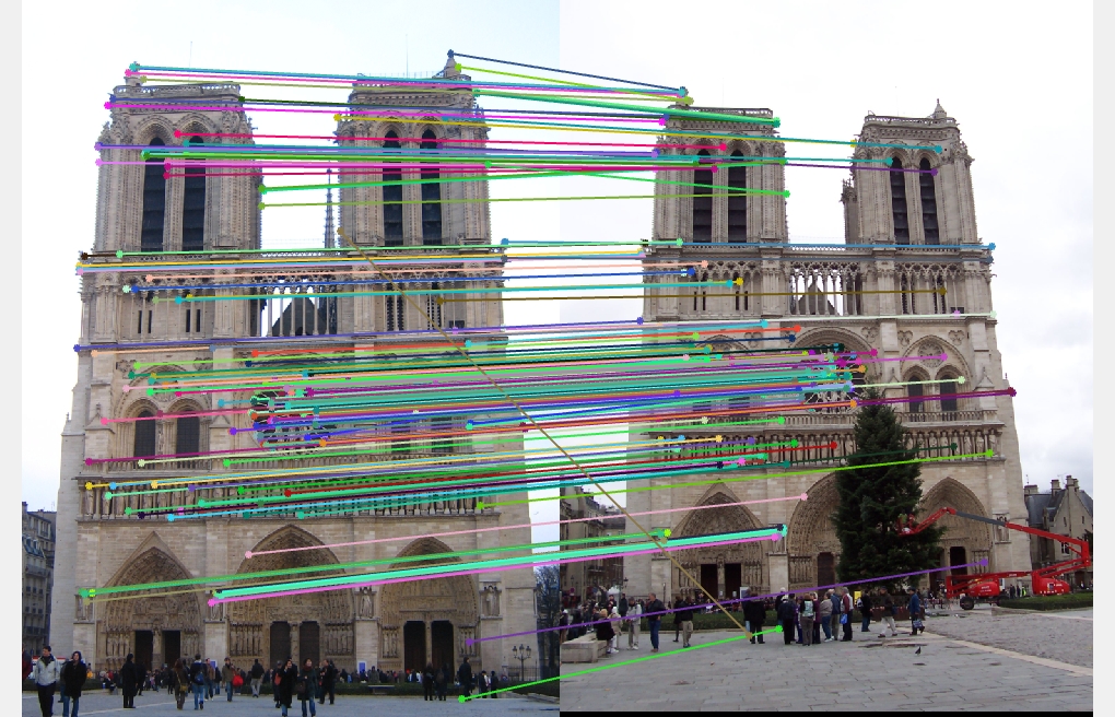
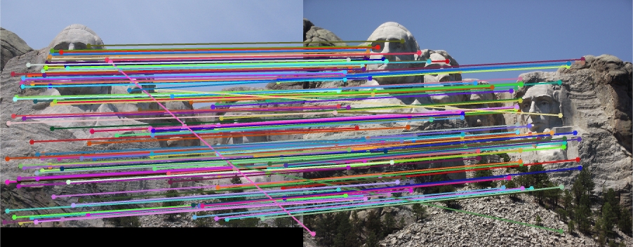
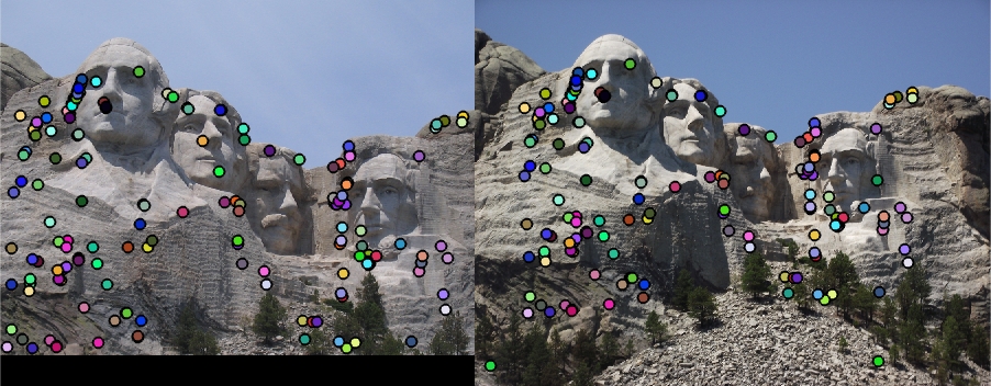
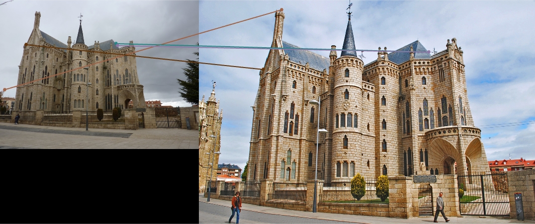
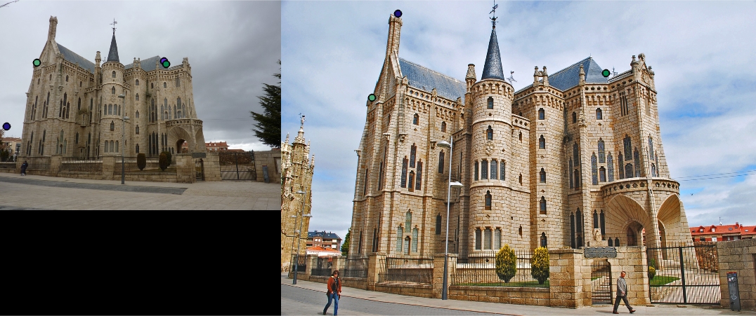
Results

The Notre Dame images were ran and there were 179 total good matches and 26 total bad matches, which means there is 87% accuracy. The Mount Rushmore images ran with even more accuracy at 92% with 144 total good matches and 13 total bad matches. This is possibly due to many more distinct features in the two images. On the other hand, the Episcopal Gaudi images ran with a very low accuracy at 25% and with low good matches at 1 and low bad matches at 3. This is because there werent many features in the beginning to even work with. This may be because of a scalability issue. The images and objects are not the same size, so there many be a problem here. Overall normalizing the features improved the accuracy by around 10% for the Notre Dame and the Mount Rushmore. In get_interest_point, using a gaussian sigma of 1.0 is actually gives an accuracy of 5% or more than using a sigma of 1.0