Project 2: Local Feature Matching

Example of a right floating element.
Overview
The goal of this assignment is to create a local feature matching algorithm using a simplified version of the famous SIFT pipeline. The pipeline consist of three parts: Harris corner detector to find interest point, a simplified version of SIFT descriptor to describe interest points, and feature matching. Additionly, I implenment Adaptive Non-maximal Suppression(ANMS) to get a more uniform distribution of interest points when only limited points are selected. And I follow the steps in Lowe's paper to build a scale-invariant interest point detector and feature descriptor. I also include the dominant direction to interest point, but due to the time limit, I did not build a rotation-invariant descriptor.
Harris Corner Dector
I follow the Algorithm 4.1 in the textbook. First comput the x,y derivatives of Gaussian, then convolve it with the image to get the gradient of the image. Then compute the products of these gradients, then convolve them with a larger Gaussian. Then use the following fomula to compute the strength of each point

Next I set a threshold to filter out weak corners. Then I find the maximum of each connect components and delete points that near the boarder of the image so the points can have a window around it.
Adaptive Non-maximal Suppression (ANMS)
The purpose of ANMS is to an even distribution of feature points across the image. The algorithm only detect features that are both local maxima and whose response value is significantly (10%) greater than that of all of its neighbors within a radius r. It does not give a better result, so I comment it out.
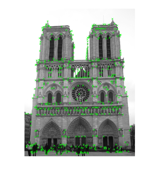 |
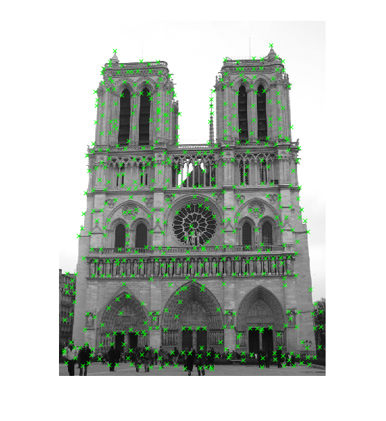 |
| 500 strongest interest points | ANMS(Top 500) |
Feature Descriptor
I implenment the SIFT descriptor described in the textbook.- compute the gradient magnitude and direction at each pixel in a 16x16 window around the detected keypoint.
- weight the gradient magnitude by gaussian.
- divid the 16x16 patch to 4x4 subpatch.
- In each 4x4 quadrant, a gradient orientation histogram is formed by (conceptually) adding the weighted gradient value to one of eight orientation histogram bins.
- Normoalize the feature vector to unit length, then chop off values over 0.2 and renormalize to unit length again.
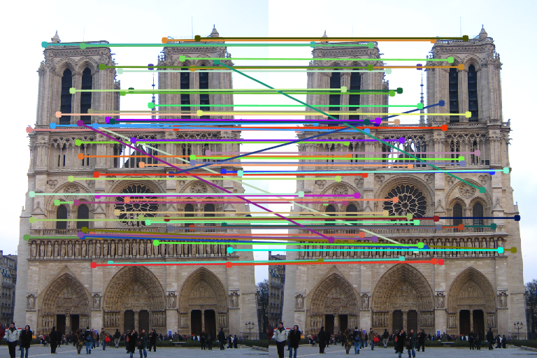
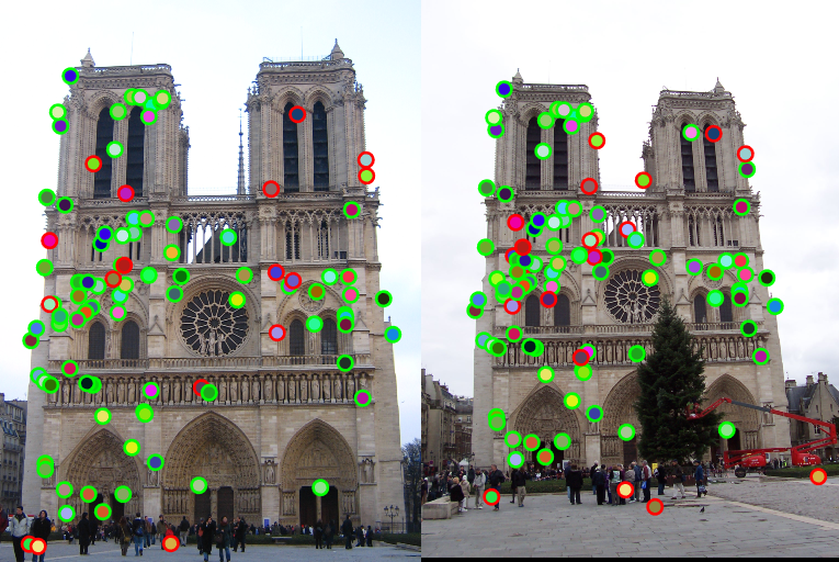
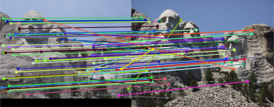
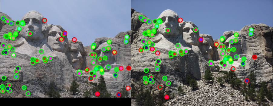
Feature Matching
I computed the distance between each descriptor of first image and each descriptor of second image. For each interest point in image one, pick the smallest and 2nd smallest distance to interest points in second image. Threshold the matches by the ratio of the two distance. Discard the matches that have large ratio which means the match is unlikely to be uniqe.
I get result of 82 good matches and 19 bad matches.
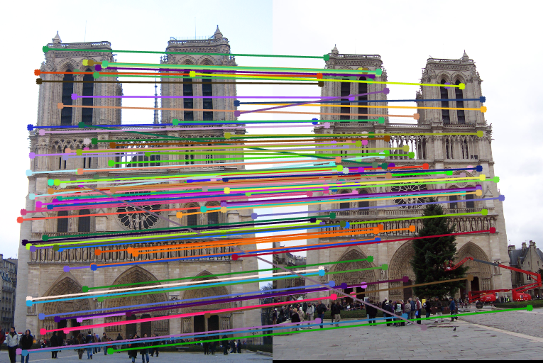
Scale-invariant feature detector and descriptor
The algorithm above has poor performance if the images have different scales.
These two image are the same image but the second is scaled by factor 0.5. For better illustration, I will rescale the second image later, but actually they are two images with different scales.
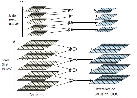
I follow the steps descripted in Lowe's paper(2004)
- Build pyramid of gaussian and pyramid of difference of gaussian.
- Find the local minimum and maximum in 3x3 neighbors in DoG pyramid.
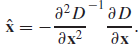
- To get real sub-pixel level extreme use this formula to shift the point
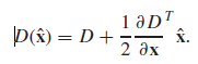
- Filter points that shifts out of boarder and weak points using formula
- Filter points that is likely to be an edge
- I used almost the same descriptor as before but get fetures in the corresponding level of pyramid

here is the result of two identical images with different scales. which is much better than original algorithm