Project 2: Local Feature Matching

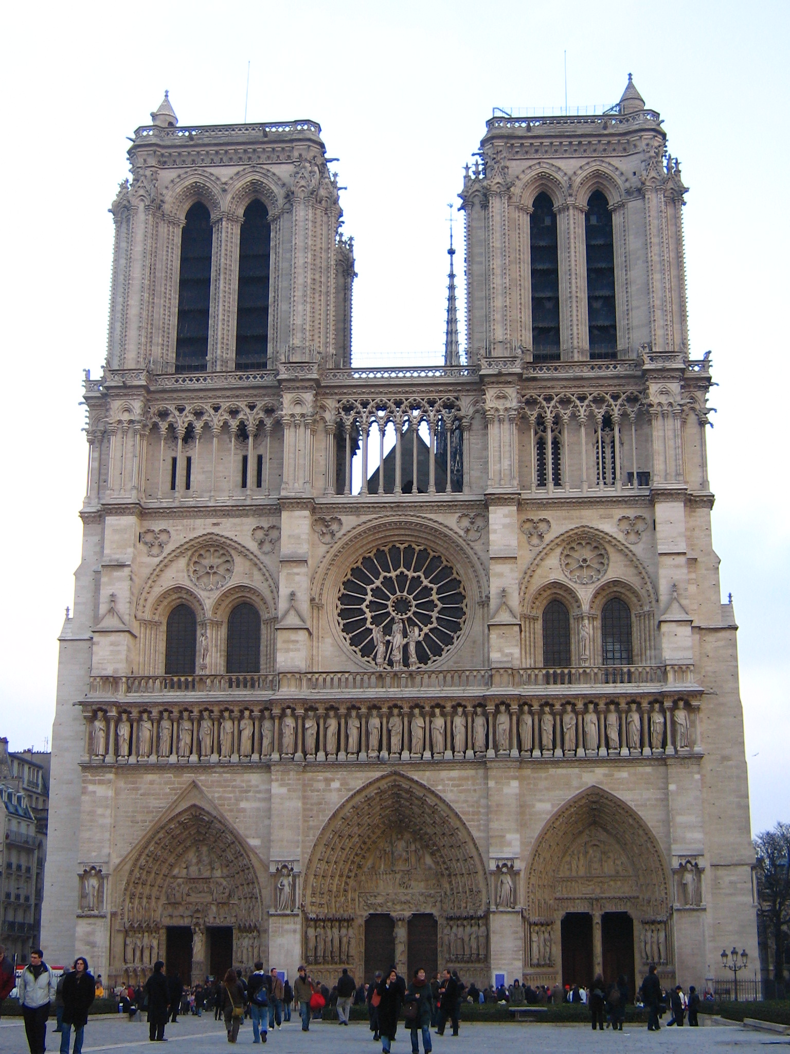
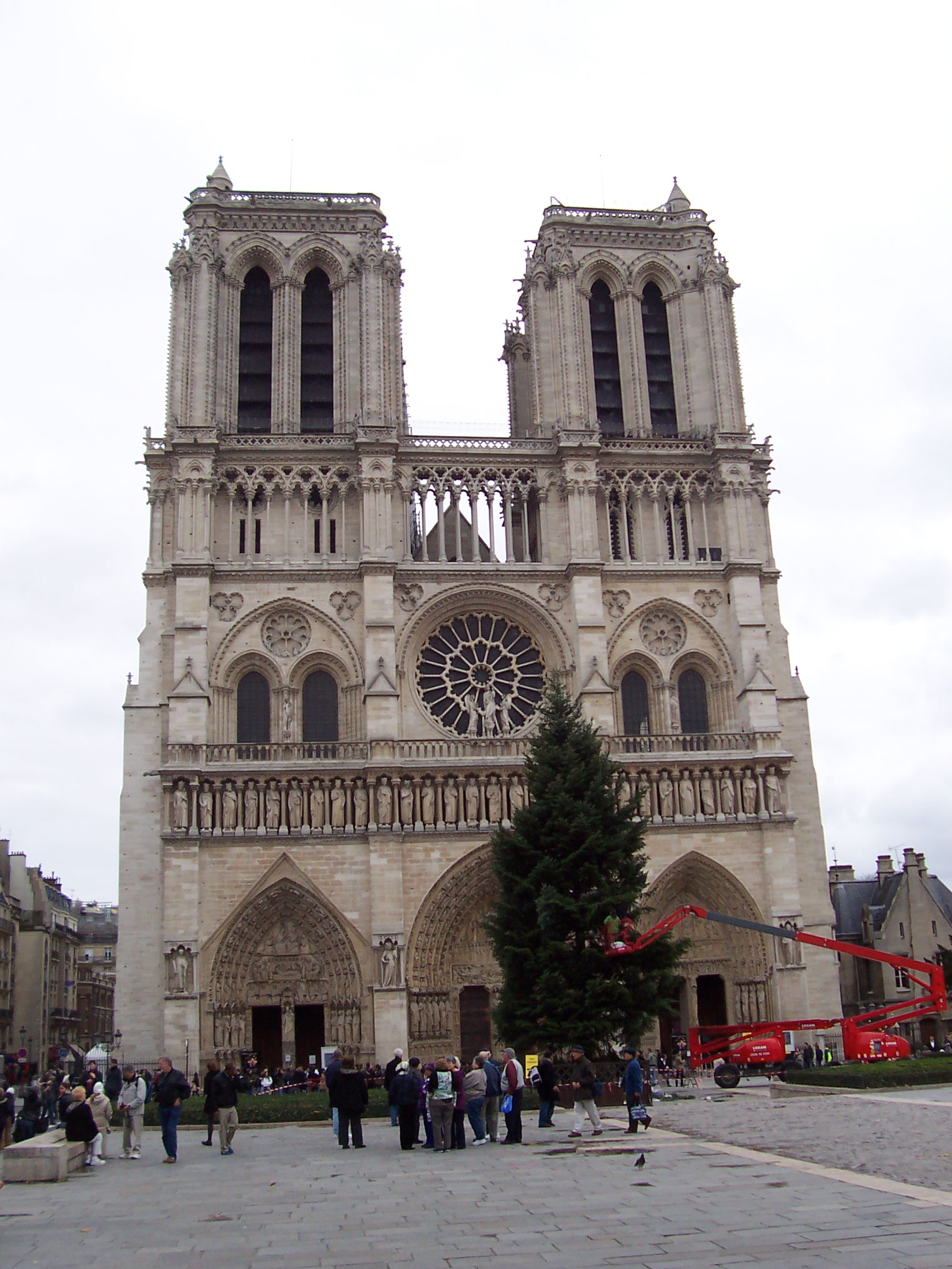
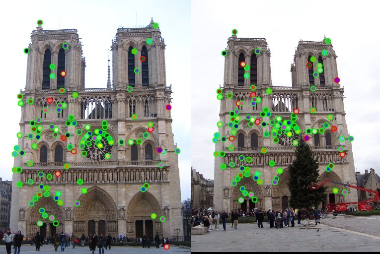
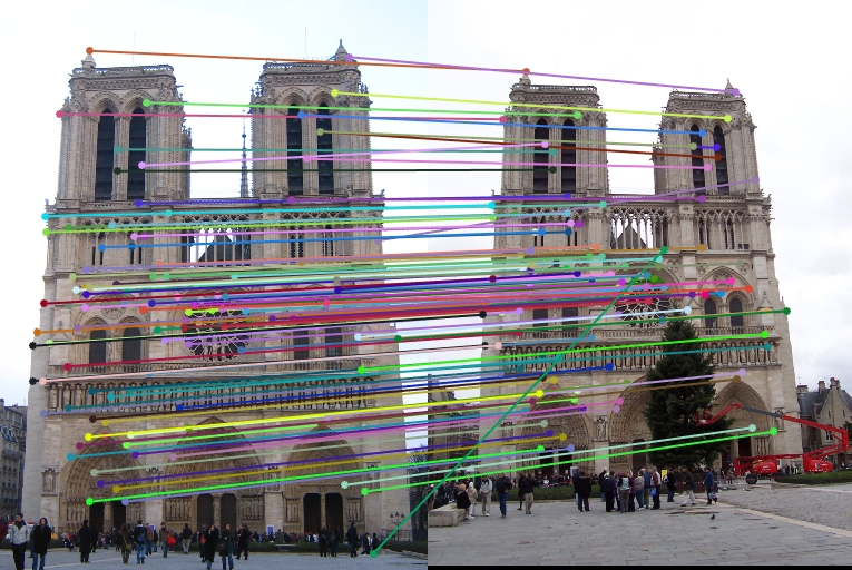
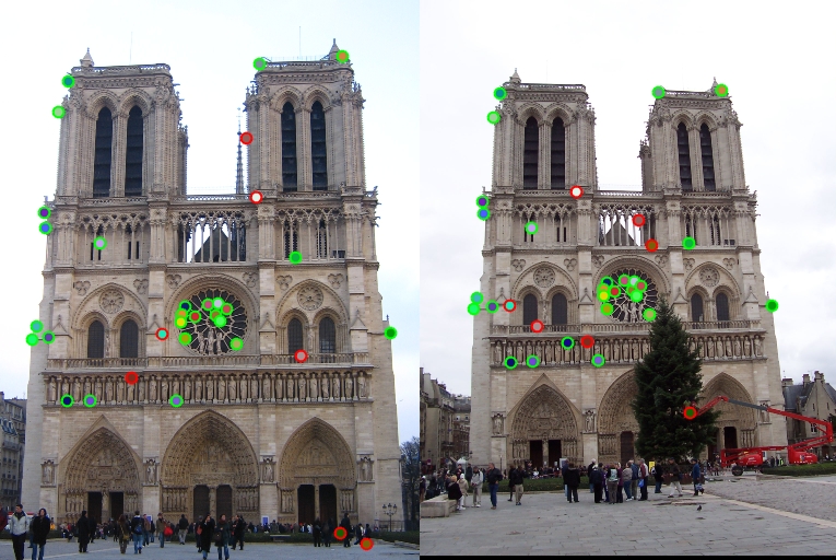
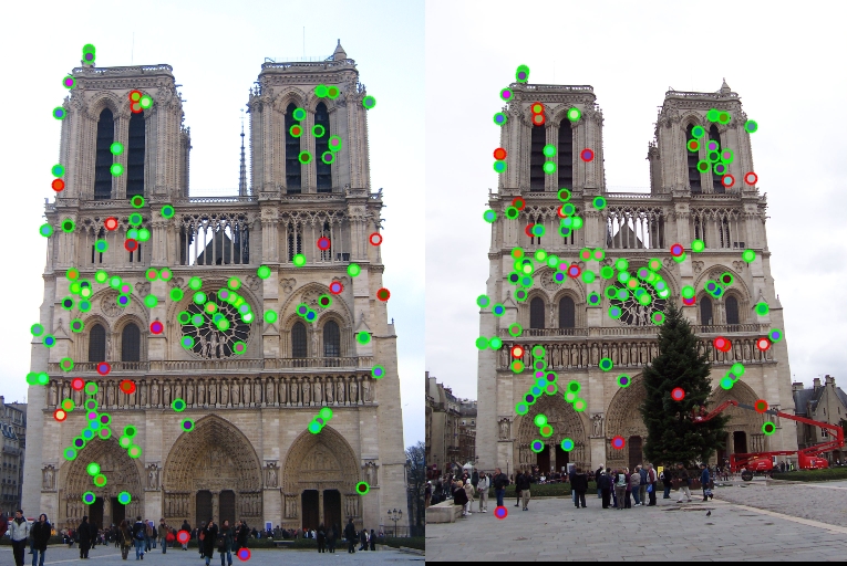
Fig.1. Example of the local feature matching results of Notre Dame pair of images.
In this project, the goal is to create an algorithm that realizes the local feature matching between a pair of images. The approach to achieve this function includes getting both images' interest points by using Harris corner detector, getting features of two images through utilizing scale invariant feature transform (SIFT) as well as matching both images' features by the use of nearest neighbor distance ratio.
This project report mainly contains three parts shown as follows:
- Get Interest Points - Harris Corner Detector
- Get Features - SIFT
- Match Features - Nearest Neighbor Distance Ratio Test
- Results
- Extra Credit
5.1. Tuning Various Parameters in Getting Interest Points
5.2. Tuning Various Parameters in SIFT
5.3. Tuning Parameters in Match Features
5.4. Extra Pairs of Images for Local Feature Matching and Discussion
1.Get Interest Points - Harris Corner Detector
Harris corner detector aims at locating key points for sparse feature matching by using local maxima in rotationally invariant scalar measures which is derived from the auto-correlation matrix. This technique uses a Gaussian weighting window making the detector response insensitive to in-plane image rotations.
The code in this part comes from get_interst_points.m. The algorithm includes the following steps and it is also shown in the following code. The first step is to compute the derivatives in both horizontal and vertical directions of the image, that is Ix and Iy, using the method of convolving the original image with Gaussians derivatives.
%% Compute the horizontal and vertical derivatives of the image Ix and Iy
Sobel_Filter_1 = [-1 0 1; -1 0 1; -1 0 1];
Sobel_Filter_2 = Sobel_Filter_1';
Ix = imfilter(image, Sobel_Filter_1);
Iy = imfilter(image, Sobel_Filter_2);
Then, three images - Ix*Ix, Ix*Iy, Iy*Iy - are required to be calculated. After this step, each of these images are needed to be convolved with a larger Gaussian to get g(Ix*Ix),g(Ix*Iy), g(Iy*Iy). In the fourth step, we need to compute a scalar interest measure using this equation:

|
Equation 1. Cornerness Function
%% Compute three images Ix*Ix, Ix*Iy, Iy*Iy
IxIx = Ix.*Ix;
IxIy = Ix.*Iy;
IyIy = Iy.*Iy;

%% Convolve each of these images with a larger Gaussian
LGaussian_Filter_Sigma = 4;
LGaussian_Filter = fspecial('gaussian', 16, LGaussian_Filter_Sigma);
IxIx = imfilter(IxIx, LGaussian_Filter);
IyIy = imfilter(IyIy, LGaussian_Filter);
IxIy = imfilter(IxIy, LGaussian_Filter);

%% Cornerness function
har= (IxIx.*IyIy-IxIy.^2) - alpha * (IxIx + IyIy).^2;
Finally, the last step is to find local maxima above a certain threshold which is set relatively low in order to get increasingly more interest points, do the non-maxima suppression and report the local maxima as detected feature point locations.
%% Find local maxima and non-maxima suppression
core_start = feature_width/2;
core_x_end = size(image,2)-core_start;
core_y_end = size(image,1)-core_start;

for i = 1 : size (har, 1)
    for j = 1 : size (har, 2)
        if har(i,j) < threshold
            har (i,j) = 0;
        end
    end
end
harwind_max = colfilt(har, [3 3], 'sliding', @max);
Maxima = har.*(har == harwind_max);
2.Get Features - SIFT

Fig.2. A schematic representation of Lowe's SIFT.
% Loop each interest point
for IP = 1:length(x)
    % Get x and y coordinate of interest point
    x_coordinate = x(IP);
    y_coordinate = y(IP);

    % Get the magnitude and direction
    x_begin = x_coordinate-feature_width/2+1;
    x_end = x_coordinate+feature_width/2;
    y_begin = y_coordinate-feature_width/2+1;
    y_end = y_coordinate+feature_width/2;
    LMag = magnitude(y_begin:y_end, x_begin:x_end);
    LDire = direction(y_begin:y_end, x_begin:x_end);

    % Smooth the magnitude
    S_Filter = fspecial('gaussian', 16, 8);
    LMag = imfilter (LMag,S_Filter);

    % Loop each grid
    Feat = zeros(1, FeatureDimensionality);
    for Grid_y = 1:4
        for Grid_x = 1:4
            x_begin_grid = 1 + (Grid_x-1)*feature_width/4;
            x_end_grid = Grid_x*feature_width/4;
            y_begin_grid = 1 + (Grid_y-1)*feature_width/4;
            y_end_gird = Grid_y*feature_width/4;
            Grid_Mag = LMag(y_begin_grid:y_end_gird,x_begin_grid:x_end_grid);
            Grid_Dire = LDire(y_begin_grid:y_end_gird,x_begin_grid:x_end_grid);
            % Loop each part of the grid
            for unit_y = 1:4
                for unit_x = 1:4
                    % Loop Binss
                    Feat =OrientationHistoBin(Bins, Grid_Dire, Grid_Mag, unit_y, unit_x, Feat, Grid_y, Grid_x);
                end
            end
        end
    end
    % Normalize every feature
    features(IP,:) = Feat(1,:)/norm(Feat(1,:));
end
The code in this part comes from get_features.m where OrientationHistoBin.m will be called. The features using Scale invariant feature transform (SIFT) are formed via computing the gradient at each pixel in a 16*16 window around the detected interest point and a Gaussian fall-off function is used to reduce the effect of gradients far from the center, as displayed in the above Fig. 2. Then, the 16*16 window is divided into various 4*4 windows. The code for this is displayed above. In each of these windows, through adding the weighted gradient value to one of the eight orientation histogram bins, a gradient orientation histogram comes into being. The code for looping through 8 bins is as follows:
function [Feat] = OrientationHistoBin(Bins, Grid_Dire, Grid_Mag, unit_y, unit_x, Feat, Grid_y, Grid_x)
EachBin = 360/Bins;
for b = 0:EachBin:EachBin*(Bins-1)
    if Grid_Dire(unit_y,unit_x) >= (b-180) && Grid_Dire(unit_y,unit_x) < (b+EachBin-180)
        index = (Grid_y-1)*4*Bins + (Grid_x-1)*Bins + (b/EachBin+1);
        Feat(1,index)  = Feat(1,index) + Grid_Mag(unit_y,unit_x);
    end
end
3.Match Features - Nearest Neighbor Distance Ratio Test
3.1. Algorithm
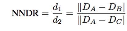
|
Equation 2. Nearest Neighbor Distance Ratio (NNDR)
% Get each distance
Distance = [];
for i = 1:size(features1,1)
    for j = 1:size(features2,1)
        Distance(i,j) = norm(features1(i,:)-features2(j,:));
    end
end

% Arrange the distances from the shortest to the longest
[Dist_Sort,I_Sort] = sort(Distance);
The last portion for local feature matching is matching the features getting from the second part. For this one, I use the nearest neighbor distance ratio test, in other words, it is to compare the distance of the nearest neighbor to that of the second nearest neighbor which these two are able to be obtained by sorting all the possible distances. This ratio is defined in the above equation and the code for getting these two nearest neighbor distances is also shown above. The code for this function is as follows:
for i = 1:size(features2,1)
    % Nearest neighbor distance ratio
    NNDR = Dist_Sort(1,i)/Dist_Sort(2,i);
    if NNDR <= 0.8
        matches(Num,2) = i;
        matches(Num,1) = I_Sort(1,i);
        confidences(Num) = 1/NNDR;
        Num = Num + 1;
    end
end
matches = matches(1:Num-1,:);
confidences = confidences(1:Num-1);
% Sort the matches so that the most confident onces are at the top of the
% list. You should probably not delete this, so that the evaluation
% functions can be run on the top matches easily.
[confidences, ind] = sort(confidences, 'descend');
matches = matches(ind,:);
4.Results
The results for the given three pairs of images are displayed below:
|
|
|
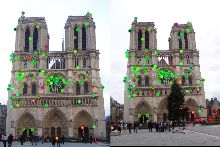
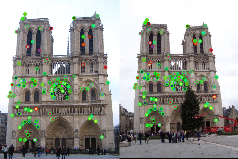
Fig.3. The results for Notre Dame - NNDR threshold: 0.8 and accuracy: 90.35 %.
|
|
|
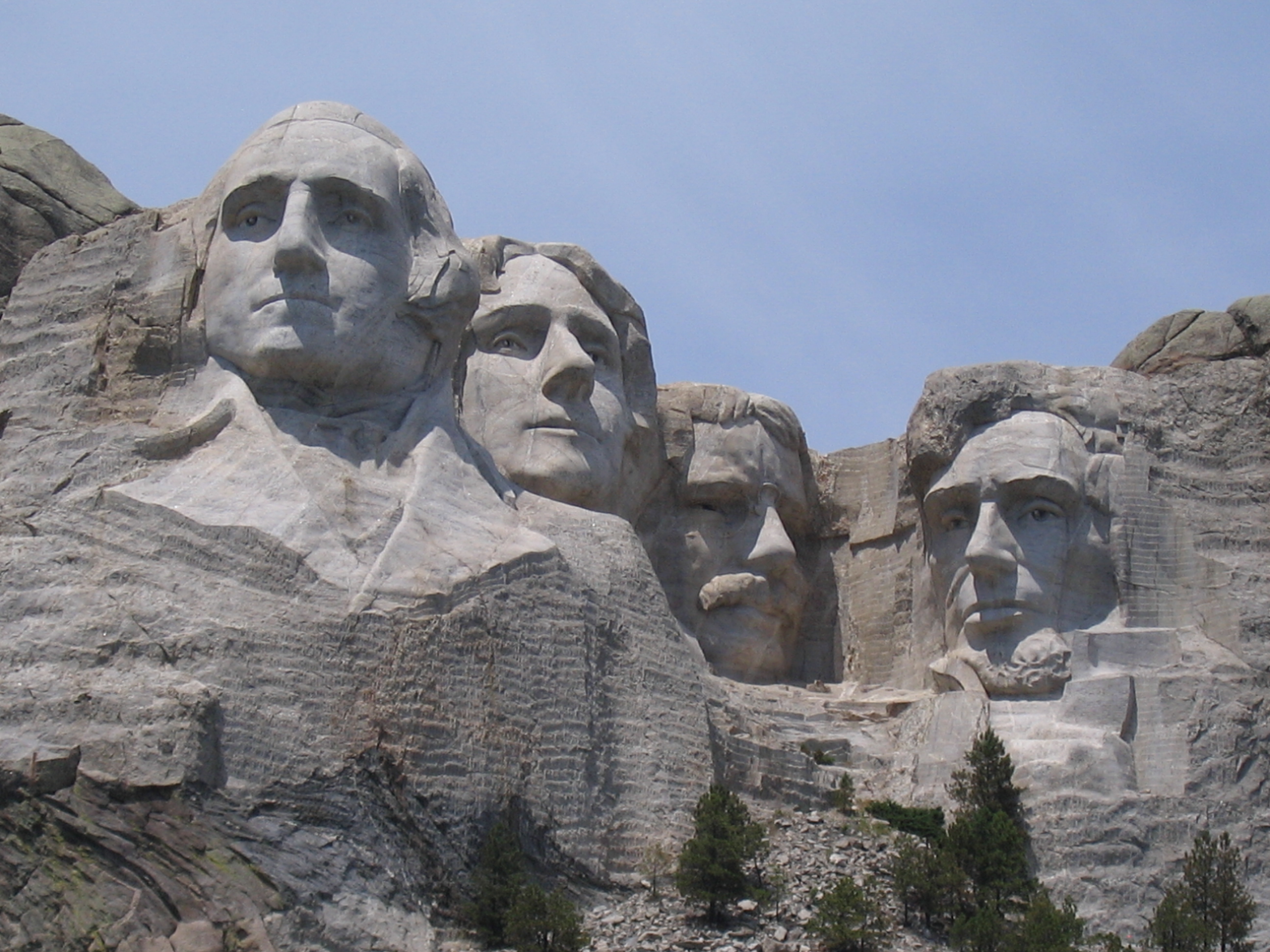
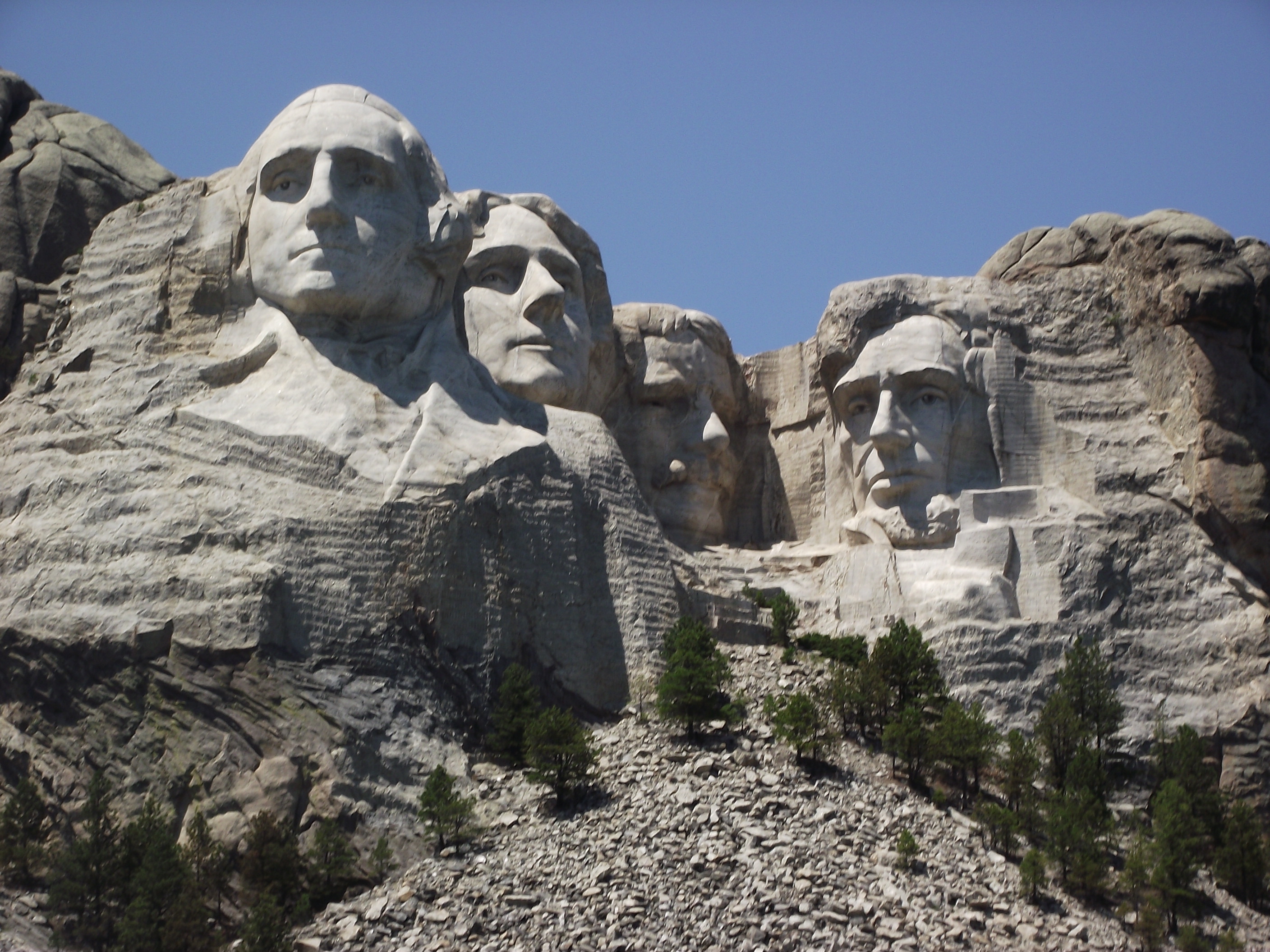
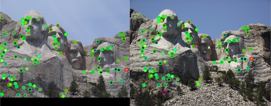
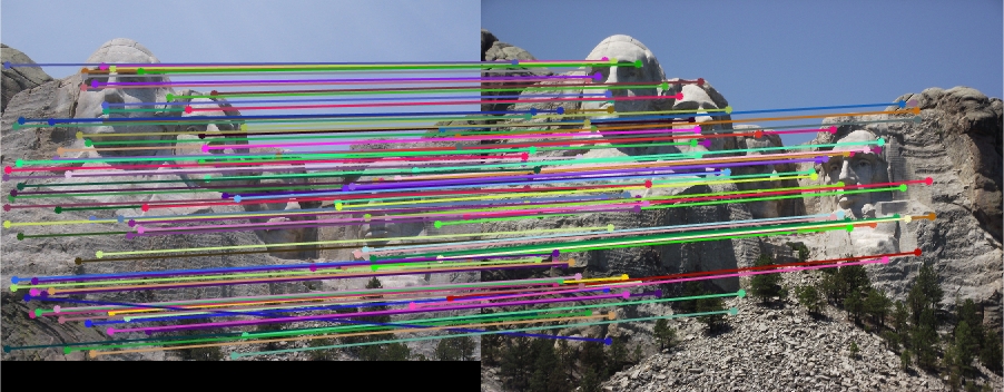
Fig.4. The results for Mount Rushmore - NNDR threshold: 0.7 and accuracy: 96.97 %
Table 1. The relationship between threshold (NNDR) and accuracy for Episcopal Gaudi pair of images.
| Threshold (NNDR) | Good Matches | Bad Matches | Accuracy |
| 0.8 | 0 | 22 | 0.00 % |
| 0.85 | 0 | 79 | 0.00 % |
| 0.9 | 8 | 257 | 3.02 % |
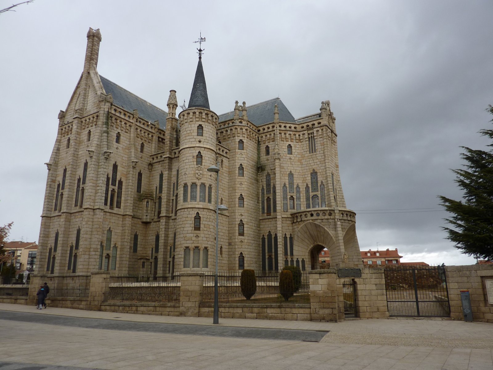
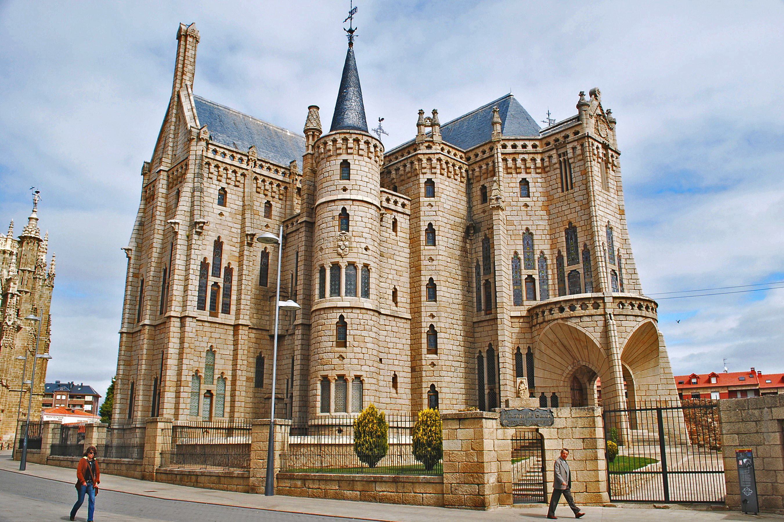
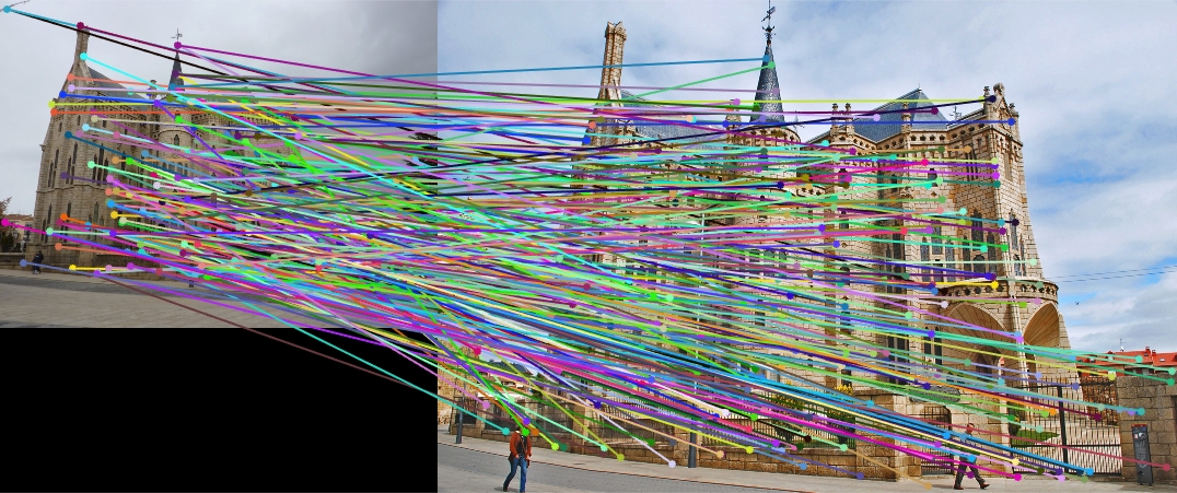
For Episcopal Gaudi pair of images, the results are not quite good. After changing several parameters, such as the threshold for NNDR as shown above in Table 4, the accuracy is still very low which means the algorithms using in this project do not work for this pair of images, likely due to the fact that these two images for local feature matching are at different intensities. The results for setting NNDR threshold as 0.9 are as follows:
|

|
|
Fig.5. The results for Episcopal Gaudi - NNDR threshold: 0.9 and accuracy: 3.02 %
5.Extra Credit
5.1. Tuning Various Parameters in Getting Interest Points
5.1.1. Threshold
Table 2. The relationship between threshold and accuracy.
| threshold | Good Matches | Bad Matches | Accuracy |
| 0.00001 | 111 | 13 | 89.52 % |
| 0.00005 | 106 | 13 | 89.08 % |
| 0.0001 | 103 | 11 | 90.35 % |
| 0.0005 | 82 | 11 | 88.17 % |
| 0.001 | 73 | 11 | 86.90 % |
| 0.005 | 41 | 8 | 83.67 % |
| 0.01 | 27 | 7 | 79.41 % |
From the above table, we can see that when the threshold is 0.0001, the accuracy is highest. It is not difficult to understand that with the decreasing of threshold from 0.01 to 0.0001, the accuracy increases since more interest points are obtained. But when the threshold is set too low, bad matches also enhance causing the accuracy to be lower. Some of the results are shown below:


|
|
|

|
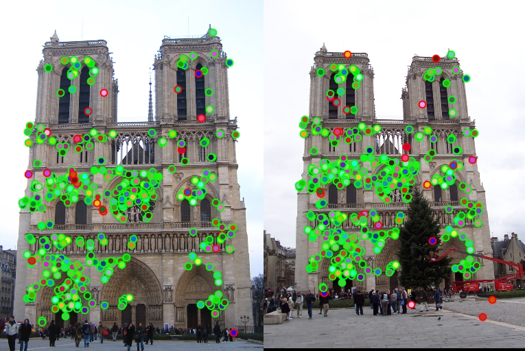
Fig.6. The original images and results for Notre Dame with NNDR threshold setting as 0.01, 0.001, 0.0001 respectively.
5.1.2. LGaussian_Filter_Sigma
Table 3. The relationship between Lgaussian_Filter_Sigma and accuracy.
| Lgaussian_Filter_Sigma | Good Matches | Bad Matches | Accuracy |
| 2 | 332 | 24 | 93.26 % |
| 4 | 103 | 11 | 90.35 % |
| 8 | 147 | 20 | 88.02 % |
By tuning the sigma of the larger Gaussian filter in the third step, we can see that with the increase of sigma, the ratio also enhances. But if we take both ratio and the number of matches into consideration, setting sigma as 4 is a good choice. The results for this are shown below:
|

|
|
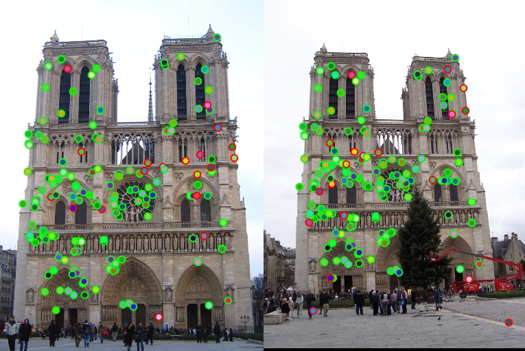
Fig.7. The results for Notre Dame with Lgaussian_Filter_Sigma setting as 2, 4, 8 respectively.
5.2. Tuning Various Parameters in SIFT
5.2.1. The number of orientation histogram bins
Table 4. The relationship between the number of bins and accuracy.
| Number of Bins | Good Matches | Bad Matches | Accuracy |
| 4 | 99 | 20 | 83.19 % |
| 8 | 103 | 11 | 90.35 % |
| 12 | 99 | 10 | 90.83 % |
| 16 | 90 | 9 | 90.91 % |
| 20 | 85 | 5 | 94.44 % |
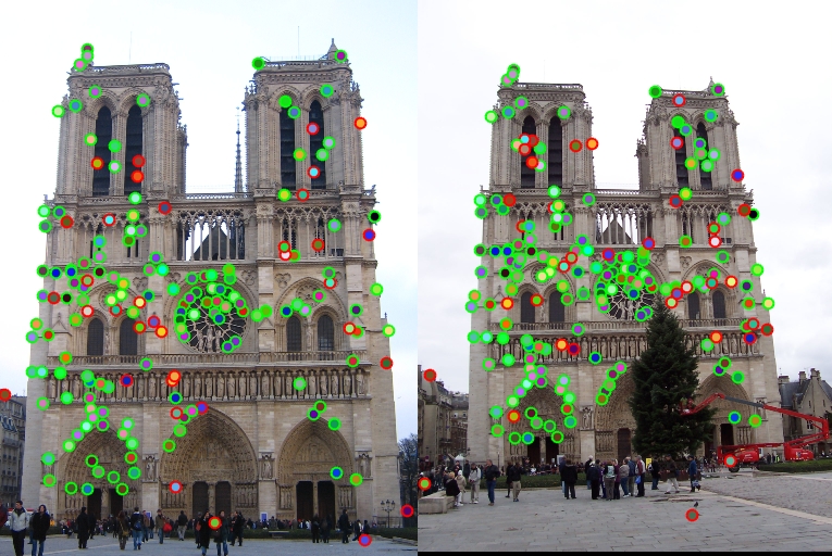
By tuning the number of orientation histogram bins, the change of the ratio emerges. As bins' number enhances, the increment of the ratio for good matches can be seen while the running time also indicates the same tendency. The outcomes are displayed below:
|

|
|

|
Fig.8. The results for Notre Dame with number of bins setting as 4, 8, 16, 20 respectively.
5.2.2. Filter for Smoothing the Magnitude- Sigma
Table 5. The relationship between sigma of the filter for smoothing the magnitude and accuracy.
| Sigma | Good Matches | Bad Matches | Accuracy |
| 4 | 107 | 19 | 84.92 % |
| 6 | 102 | 13 | 88.70 % |
| 8 | 103 | 11 | 90.35 % |
| 10 | 103 | 11 | 90.35 % |
| 12 | 102 | 10 | 91.07 % |
This is able to be easily seen that the accuracy is enhanced with the increment of sigma in the filter utilized to smooth the magnitude. But when sigma is increased from 4 to 12, the increment of the accuracy is only about 6 %. In other words, the change is not that evident.
5.2.3. Filter at the Beginning for Image - Sigma
Table 6. The relationship between sigma of the beginning filter for image and accuracy.
| Sigma | Good Matches | Bad Matches | Accuracy |
| 0.5 | 78 | 4 | 95.12 % |
| 1 | 103 | 11 | 90.35 % |
| 1.5 | 128 | 25 | 83.66 % |
| 2 | 136 | 49 | 73.51 % |
For the filter used to smooth the image, when I change the sigma of it from 0.5 to 2, the accuracy changes a lot for about 22 % as compared to the change above for the smooth magnitude filter.
5.3. Tuning Parameters in Match Features
5.3.1. Threshold for NNDR
Table 7. The relationship between threshold for NNDR and accuracy.
| Threshold (NNDR) | Good Matches | Bad Matches | Accuracy |
| 0.7 | 44 | 2 | 95.65 % |
| 0.75 | 75 | 4 | 94.94 % |
| 0.8 | 103 | 11 | 90.35 % |
| 0.85 | 147 | 38 | 79.46 % |
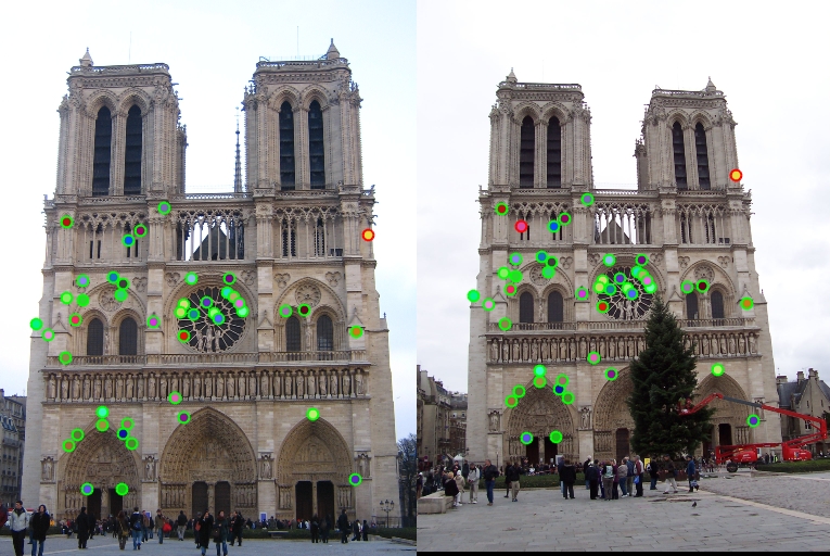
From the above Table 3, it can be easily seen that with the decrease of threshold, the ratio increases but at the same time the number of matches drops. Thus, it seems that in this case, setting the threshold as 0.8 is better when considering both the number of matches and ratio. The results are as follows:
|

|

|
|
Fig.9. The results for Notre Dame with NNDR threshold setting as 0.70, 0.75, 0.80, 0.85 respectively.
5.4. Extra Pairs of Images for Local Feature Matching and Discussion
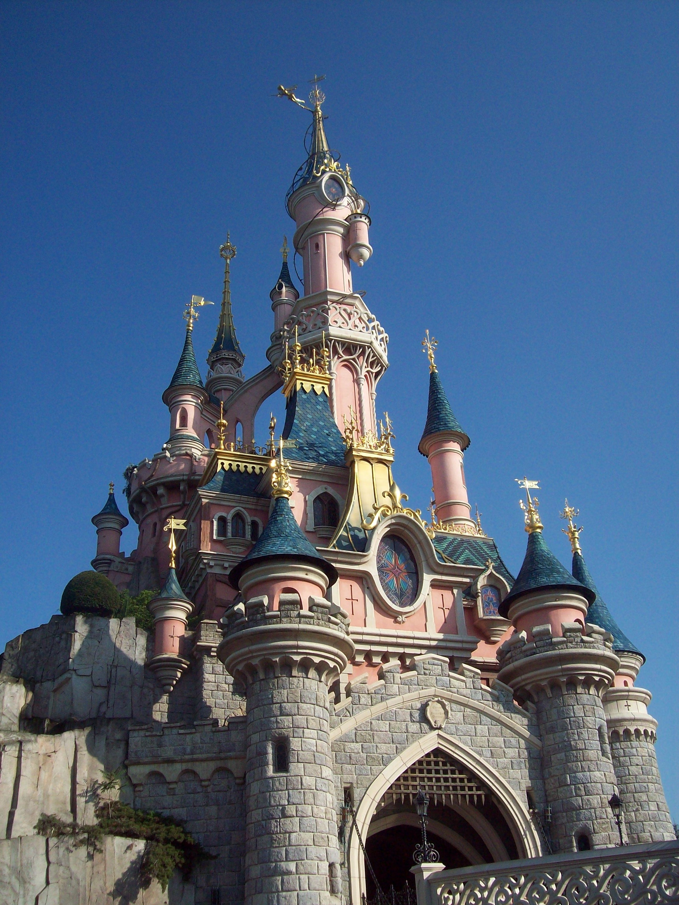
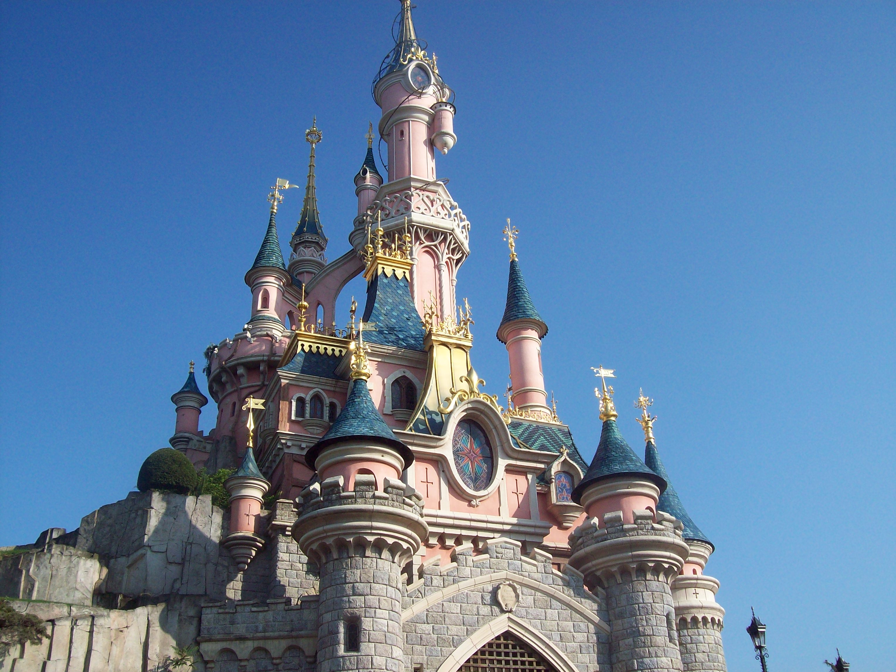
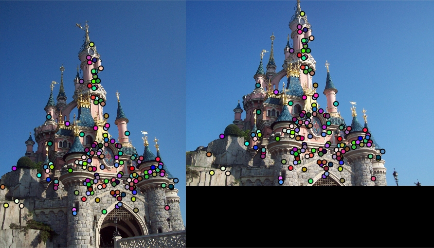
5.4.1. Sleeping Beauty Castle Paris
|
|
|
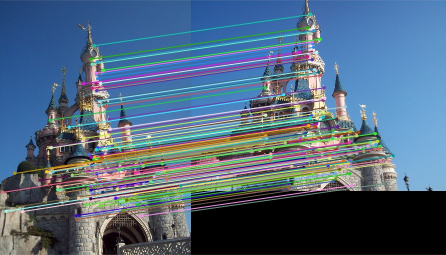
Fig.10. The results for sleeping beauty castle paris.
It can be seen from the above results of figures that the local features of the two images are matched very perfectly indicating the effectiveness of the algorithms using in this project.
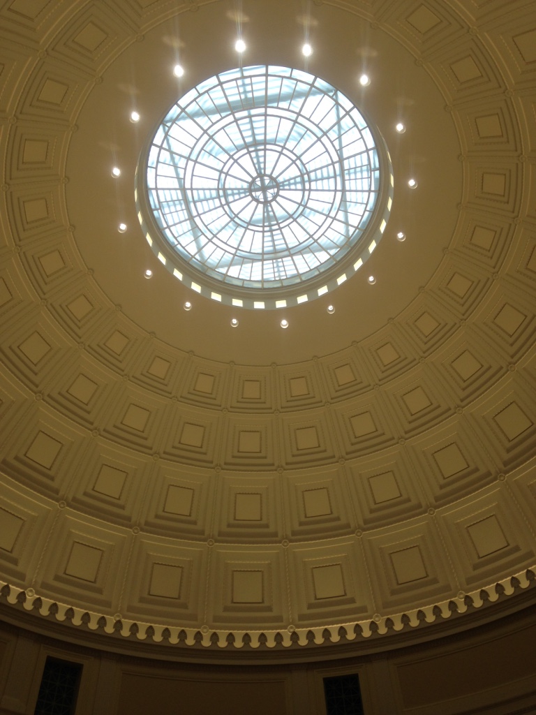
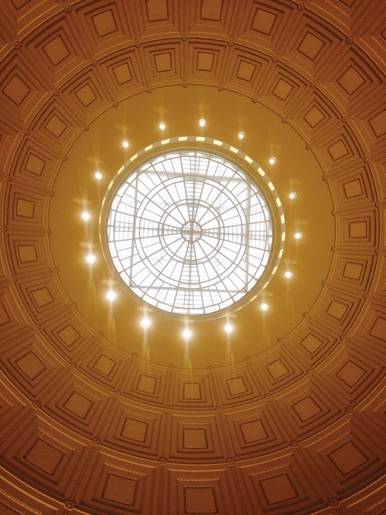
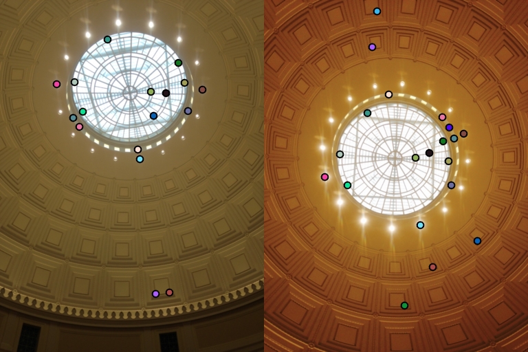
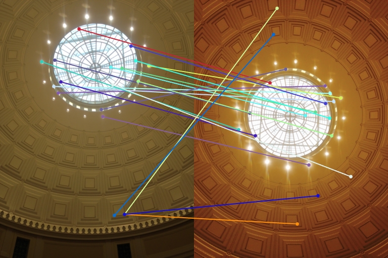
5.4.2. MIT Library Ceiling
|
|
|
Fig.11. The results for the ceiling in MIT library.
The results for this pair of images seem not quite good which may owe to the fact that many local features are very similar.
5.4.3. Boston New Year
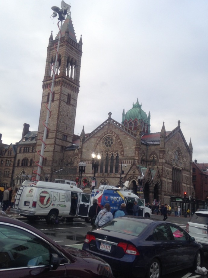
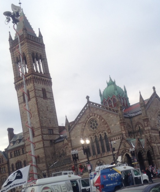
|
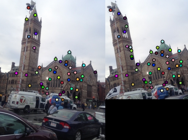
|
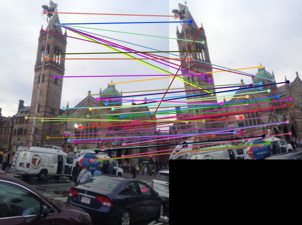
|
Fig.12. The results for the pair of images taken at Boston during New Year.
For this pair of images, even these two images are taken at different angles and different distances, the accuracy of local feature matching is quite satisfactory approximately above 80 % except a few of mismatches due to similarity.
Thanks for watching. This is all my work for CS 6476-Project 2-Local Feature Matching. I really appreciate your time. If you have any problem, please contact me and my email address is xwu72@gatech.edu.