Xiaobin Xiong

Project 2: Local Feature Matching

Content

1. Overview
2. Implementation
3. Results and discussion
4. Extra credits attempted

1. Overview

A local feature matching algorithm on instance-level is implemented in this assignment to match same physical scenes from multiple views. Using simplified versions of the famous SIFT pipeline, the algorithm could first detect interest points in get_interest_points.m . Then the local feature is described in each interest point in get_features.m. Finally, feature matching is realized in match_features.m. 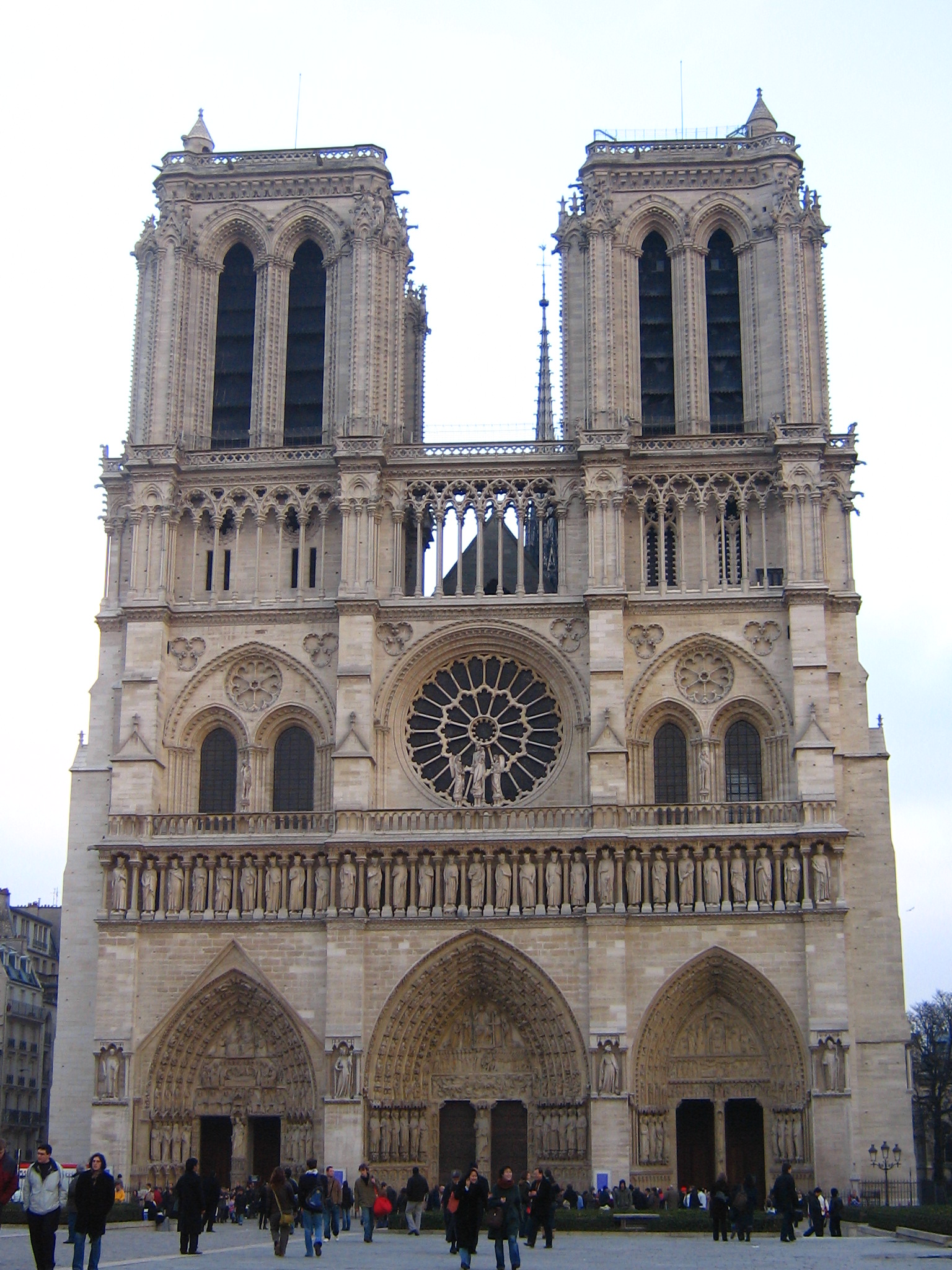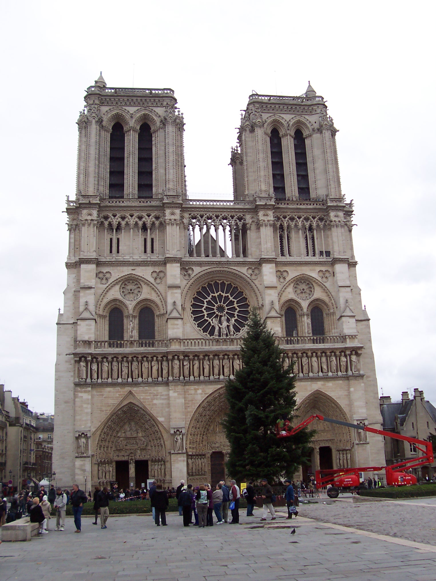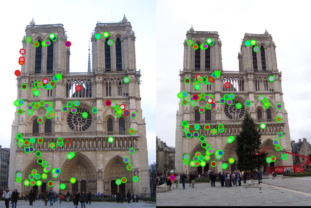Simple implementations are experimented first and then more sophisticated algorithms are adapted to increase the successful match rate. Fig. 1 shows the Notre Dame image pair on which we will match features.

2. Implementation

1. Interest point detection

Harris corner detector is implemented in get_interest_points.m. The second moment matrix is used to approximate local auto-correlation which represents distinctiveness. To calculate the second moment matrix, Sobel-like filter is used to calculate the gradients in both x- and y- directiones. A gaussian filter is applied on each element of the matrix.

[rows,cols] = size(image);
Xfilter = [-1,0,1;-1,0,1;-1,0,1];
Yfilter = Xfilter';
Ix = imfilter(image,Xfilter);
Iy = imfilter(image,Yfilter);
gauss = fspecial('gaussian');
Ix2 = imfilter(Ix.^2, gauss);
Iy2 = imfilter(Iy.^2, gauss);
Ixy = imfilter(Ix.*Iy,gauss);

Then we can calculate the cornerness score using the suggested alpha = 0.06. Then Matlab colfilt function is applied to assign local maximum score to each pixel. The local window size is determined by feature_width, which is an input value for this function.

alpha = 0.06;
harris = (Ix2.*Iy2 - Ixy.^2) - alpha*((Ix2+Iy2).^2);
maxi = colfilt(harris,[feature_width,feature_width],'sliding',@max);

Setting up a threshold for the cornerness score, we can select best local corners among all the corners in the image. The threshold matters. If it is too high, only a few corners can be detected, which could only give few features for matching. If the threshold is to low. The too much corners are detected and would decrease efficiency. Experimentally, good thresholds can be easily found. As physical scenes are taken from multiple views, interest points near the boundaries would be hard to find matches. Detected interest points near boundaries are surpressed.

threshold = 0.0003;
extracted = (harris==maxi) & (harris > threshold);
boundaryX = 5*feature_width;
boundaryY = 5*feature_width;
[y, x] = find(extracted(boundaryY:rows-boundaryY,boundaryX:cols-boundaryX));
y = boundaryY + y - 1;
x = boundaryX + x - 1;

1. Local feature description

A SIFT-like local feature description is realized in get_features.m. Given an interest point, locally we find a 16x16 matrix and divide it into 4x4 section equally. For each section, the gradients are distributed over a histogram on gradient directions. The histogram is chosen to be of size 8. Then at each interest point, we have a 4x4x8 = 128 dimensional vector.

As the interest point could be at the boundaries in general cases (not in get_interest_points.m), the input image is padded first. imgradient function is used to calculate the image gradients Gmag and directions Gdir on pixel level. Local gradient matrix and gradient direction matrix are stored in local and local_dir respectively. Then histograms at all the sections are calculated.

half = feature_width/2;
quad = feature_width/4;
image = padarray(image,[half,half]);

[Gmag,Gdir] = imgradient(image);

x = x + half;
y = y + half;
dim_x = size(Gmag,2);
dim_y = size(Gmag,1);
for i = 1:length(y)
    x(i) = round(x(i));
    y(i) = round(y(i));
    local = Gmag(y(i)-half:y(i)+half-1,x(i)-half:x(i)+half-1);
    local_dir = Gdir(y(i)-half:y(i)+half-1,x(i)-half:x(i)+half-1);
    current_feature = [];
    for j = 0:3
        for k = 0:3
            temp_grad = local(1+quad*j:quad*(j+1),1+quad*k:quad*(k+1));
            temp_dir = local_dir(1+quad*j:quad*(j+1),1+quad*k:quad*(k+1)) + 180;
            temp_grad = reshape(temp_grad,[16,1]);
            temp_dir = reshape(temp_dir,[16,1]);
            temp_dir = floor(temp_dir/45)+1; 
            hist_count = zeros(8,1);
            for count = 1:16
                hist_count(temp_dir(count),1) = hist_count(temp_dir(count),1) + temp_grad(count);
            end
            hist_count = hist_count/sum(hist_count);
            current_feature = [current_feature;hist_count];
        end
    end
    coord = [x(i)/dim_x;y(i)/dim_y]*coord_factor;
    current_feature = [current_feature;coord];
    current_feature = current_feature/norm(current_feature,2);
    features(i,:) = current_feature';
end

1. Feature Matching

Given two sets of features extracted from images of two different views, we would want to match features across the images. Each feature is a high dimensional vector (128 dimensional for abovementioned algorithm). Euclidean distance is the only used metric. For each feature in image 1, all the features in image 2 would be iterated to calculate the Euclidean distances to the feature in image 1 and save the distances in a vector called feature_dist. The feature in image 2 which has the smallest distance nearest to the feature in image 1 is the match. And the second smallest distance second_nearest is used to calculate the confidence. If second_nearest is much bigger than nearest, then the matched feature is more likely to be a right match. Thus confidence is calculated by 1-nearest/second_nearest. Sorting the matches based on the confidence scores we can select matches with higher confidence scores. With generating more than 100 features in each image, top 100 matches will be selected to be the output for match_features.m.

num_features = min(size(features1, 1), size(features2,1));
matches = zeros(num_features, 2);
AllPossMatch = [];
for i = 1:size(features1,1)
    feature_dist = [];
    for j = 1:size(features2,1)
        feature_dist =[feature_dist; norm(features1(i,:) -features2(j,:))];
    end
    [nearest,pos] = min(feature_dist);
    feature_dist(pos) = [];
    second_nearest = min(feature_dist);
    confidence = 1 - nearest/second_nearest;
    AllPossMatch = [AllPossMatch;[i,pos,confidence]];
end
confidences = AllPossMatch(:,3);
[confidences, ind] = sort(confidences, 'descend');
sorted_matches = AllPossMatch(ind,1:2);
matches = sorted_matches(1:num_features,:);
matches = matches(1:100,:);

3. Results and Discussion

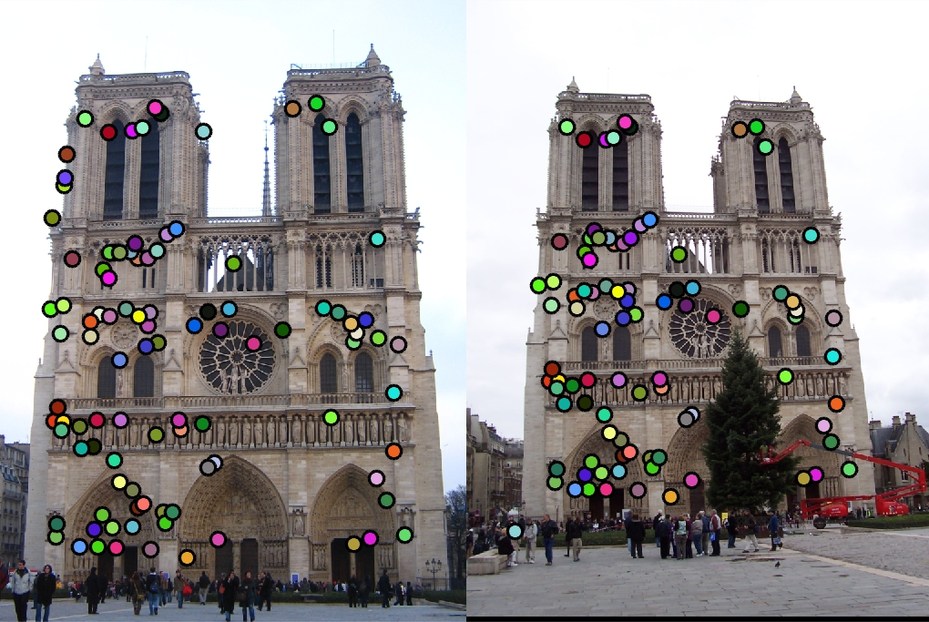
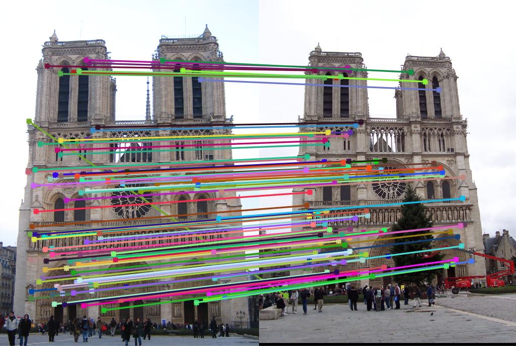
Using the abovementioned algorithms, we first match the features in the Notre Dame image pair and reach to 88% accuracy using threshold = 0.0003 in get_interest_points.m. This results is shown in Fig. 2 taking as baseline. Lowering the threshold = 0.000001 will also increase the match accuracy up to 2% (90%). Note that, bad matches actually happens in the case that multiple features in image 1 are matched to the same feature in image 2, which is not ideal. Feature should be matched individually, meaning each feature should have only one match. To resolve this issue, each multiple matched feature should be detected. And the according best match (with highest confidence) is saved. The other misleading match indexes are saved to abandonList and then got deleted in the AllPossMatch matrix.

abandonList = [];
[match2,index] = sort(AllPossMatch(:,2),'descend');
maxConf = 0;maxIndex = 1;
for i = 2:size(match2)
    if match2(i) == match2(i-1)
        maxConf = max([maxConf,AllPossMatch(index(i),3), AllPossMatch(index(i-1),3)]);
        if maxConf > max([AllPossMatch(index(i),3), AllPossMatch(index(i-1),3)])
            abandonList = [abandonList,index(i)];
        elseif maxConf == AllPossMatch(index(i),3)
            abandonList = [abandonList,index(maxIndex)];
            maxIndex = i;
        else
            abandonList = [abandonList,index(i)];
        end
    else
        maxConf = 0;
        maxIndex =i;
    end
end
AllPossMatch(abandonList,:) = [];

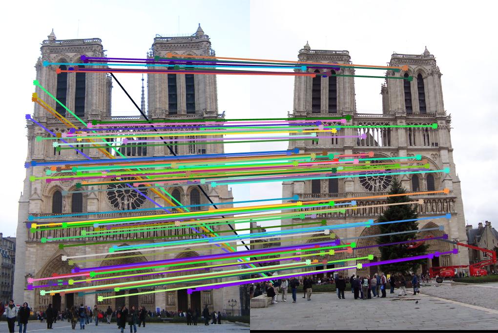
Having this in match_features.m, the accuracy reaches to 98%. Fig. 3 shows the matching results.

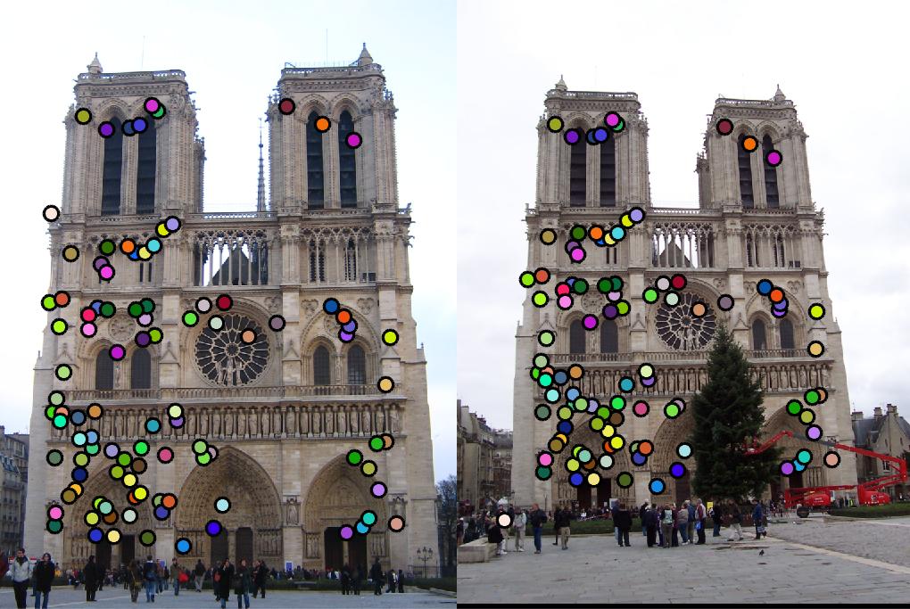
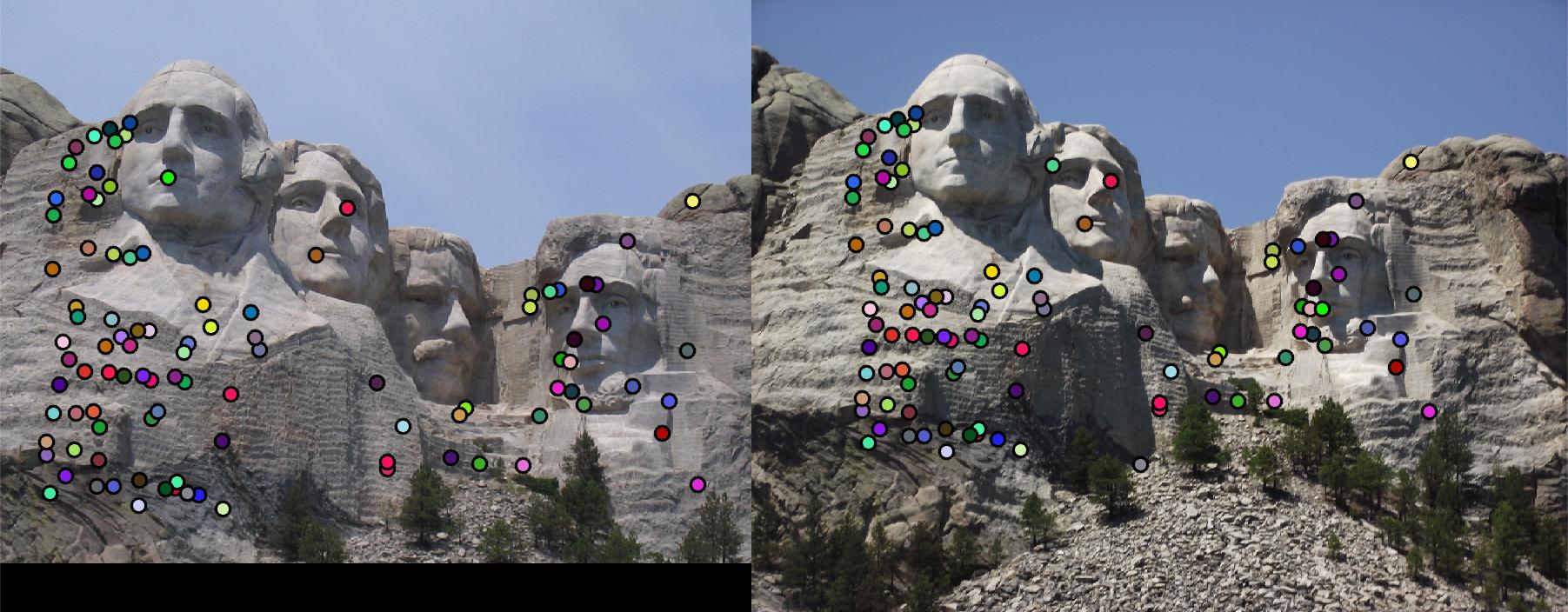
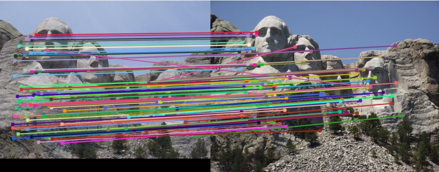
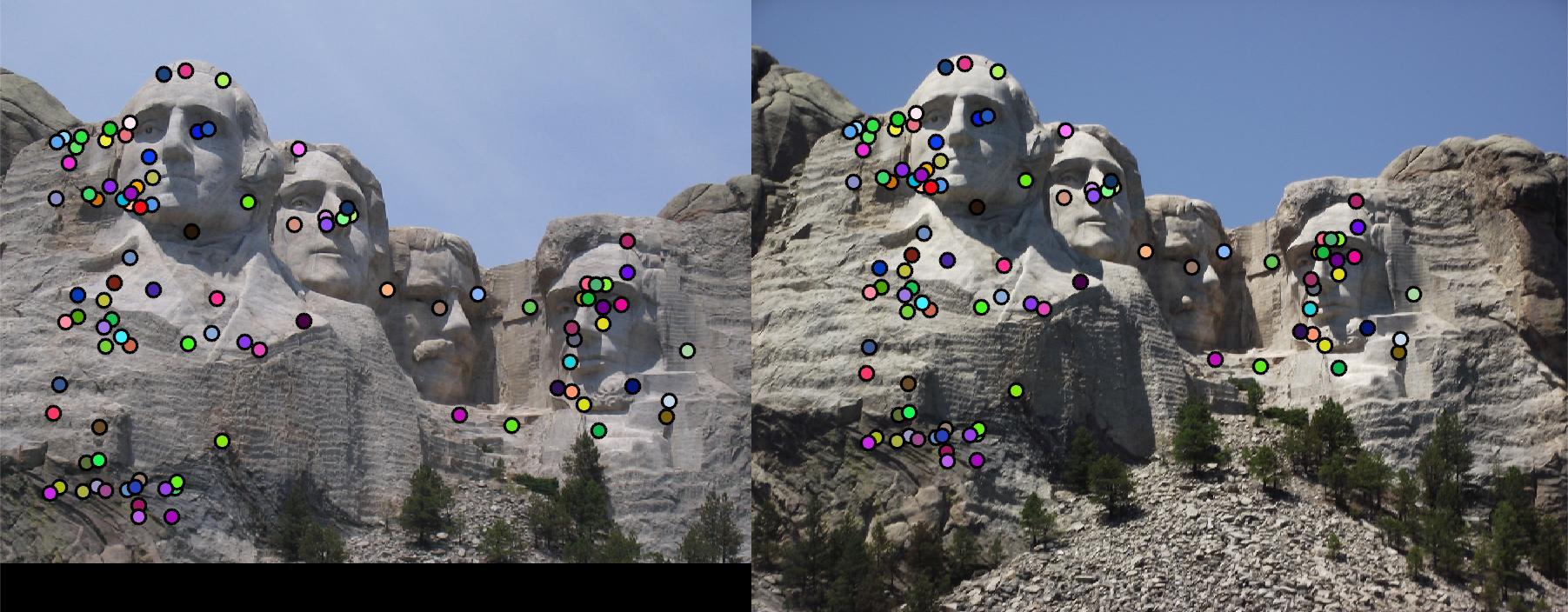
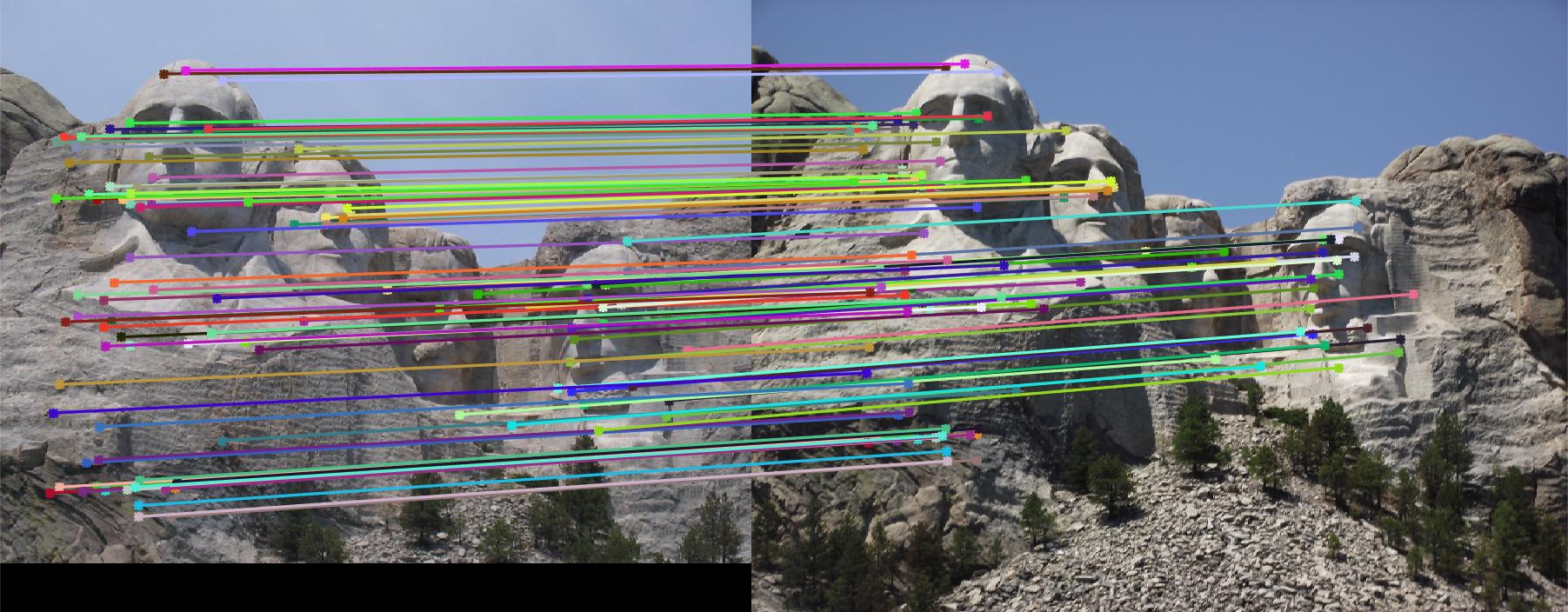
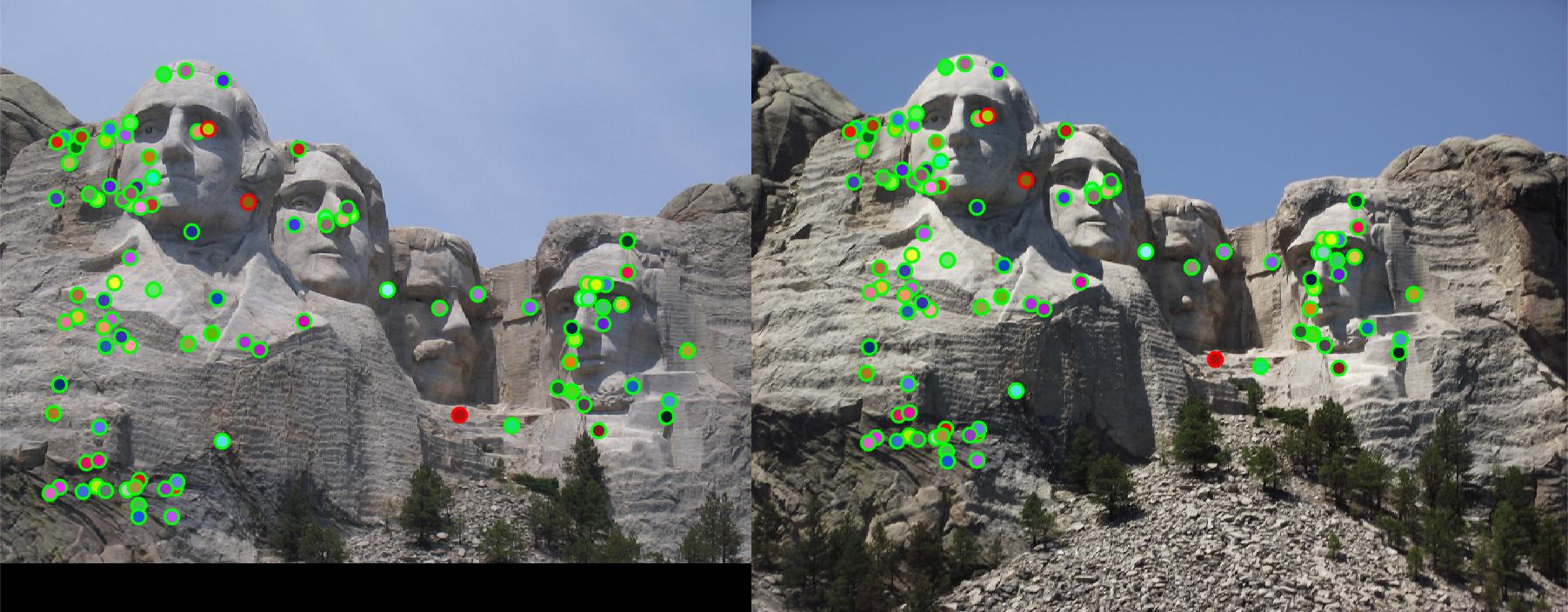
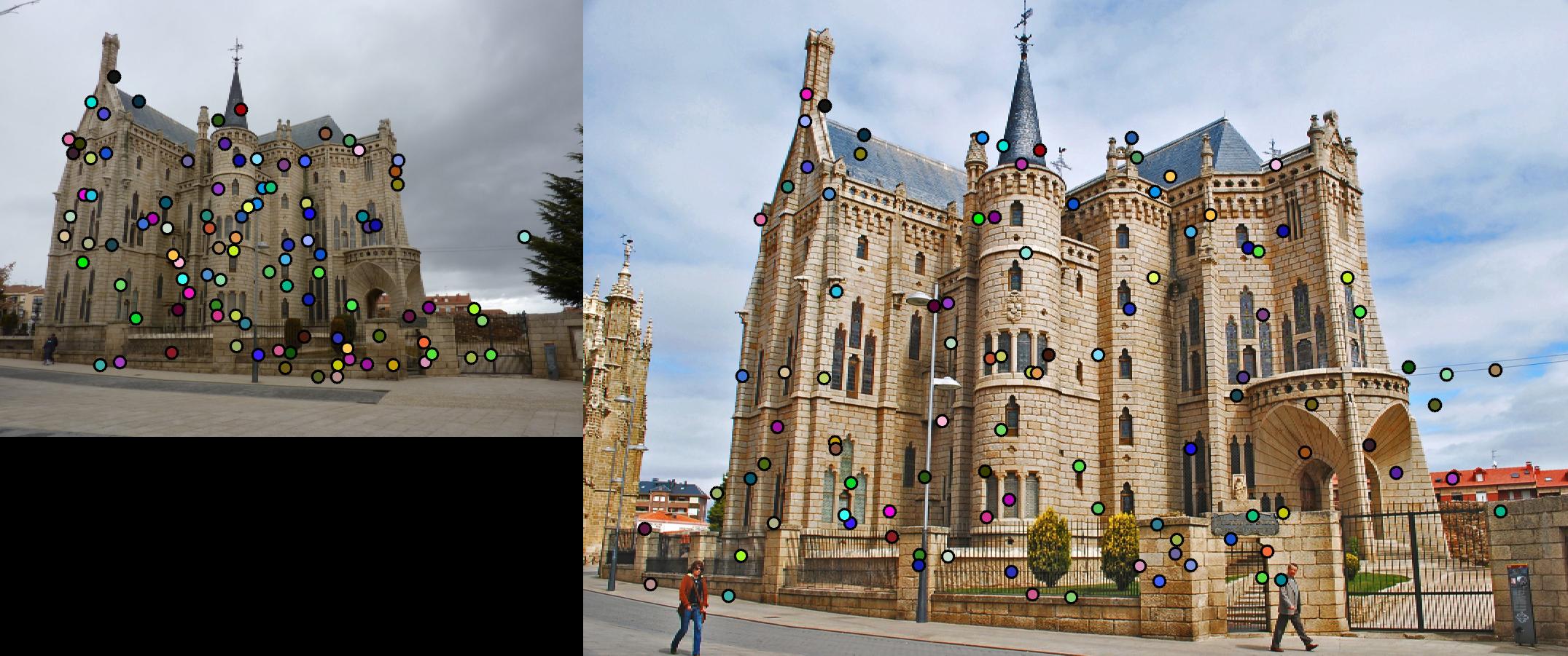
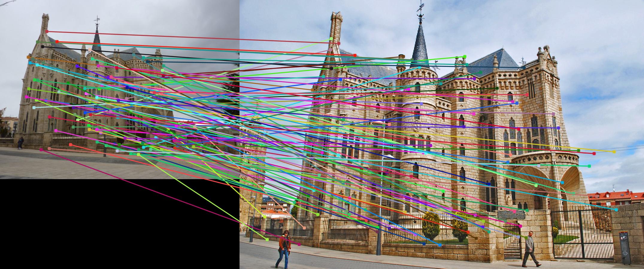
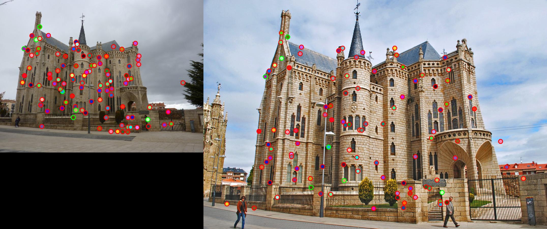
Let threshold = 0.0003, and use the same code to run feature matching on Mount Rushmore pair. 92% accuracy is achieved. Fig. 4 shows the match result. However, due to strong similarity of the corners in Episcopal Gaudi pair, accuracy is quite low, results of which show in Fig. 5.

4. Extra credits attempted

As the baseline implementation results high accuracy for Notre Dame pair already, the Mount Rushmore pair will be used for examining the extra credit.

1. Keypoint Orientation Estimation: 5pts

When detecting interest point in Harris corner detector, we can also estimate local orientation for each interst point. Saving the local orientation in vector orientation, we can further generate local feature rotation invariant. ls is the local orientation calculator size. For the Mount Rushmore pair, 20 is the relative good size, increasing the accuracy from 92% to 97%. The full implementation is in get_interest_points_extra.m .

orientation = zeros(length(x),1);
ls = 20;
[Gmag,Gdir] = imgradient(image);
for i = 1:length(x)
    local_ori_matrix = Gdir(y(i)-ls:y(i)+ls-1,x(i)-ls:x(i)+ls-1);
    orientation(i) = sum(sum(local_ori_matrix))/(2*ls)/(2*ls);
end

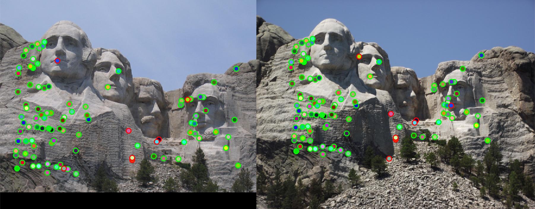
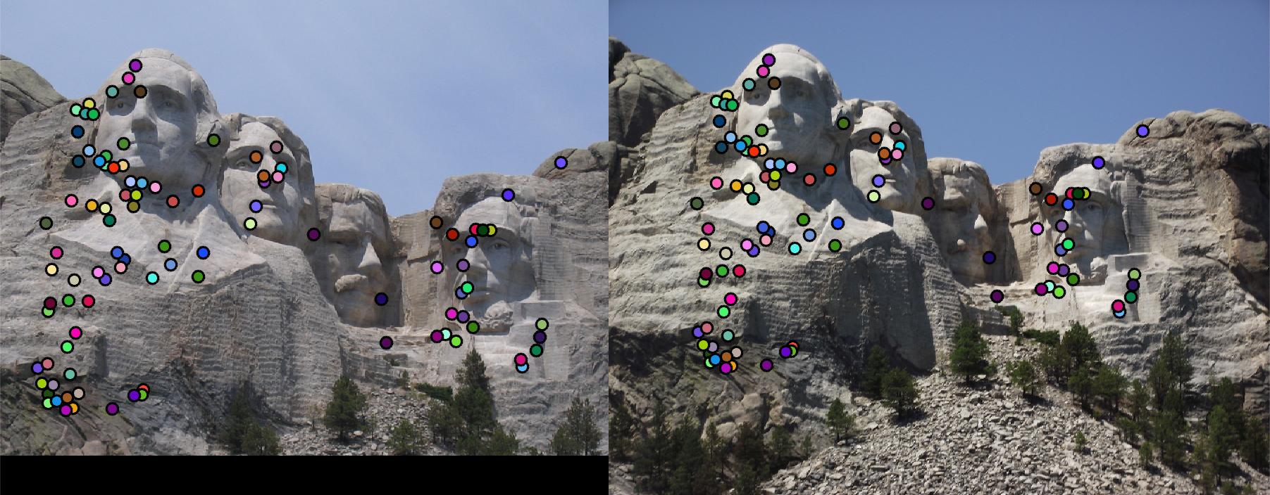
1. Local Feature Descriptor with rotation invariance: 5pts

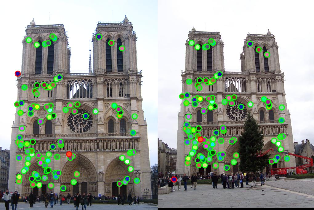
As get_interest_points_extra.m can estimate orientation, the local feature descriptor should also have rotational invariance. Simply add the orientation at each interest point to the local gradient direction matrix, and then limit the range of local direction to [0,2pi]. Full implementation is in get_features_extra.m. Fig. 6 shows the Mount Rushmore pair using this local feature descriptor with rotation invariance. Accuracy is increased to 97%.

local_dir = local_dir + orientation(i);
local_dir = local_dir + 360*(local_dir<0); 
local_dir = local_dir - 360*(local_dir>360);

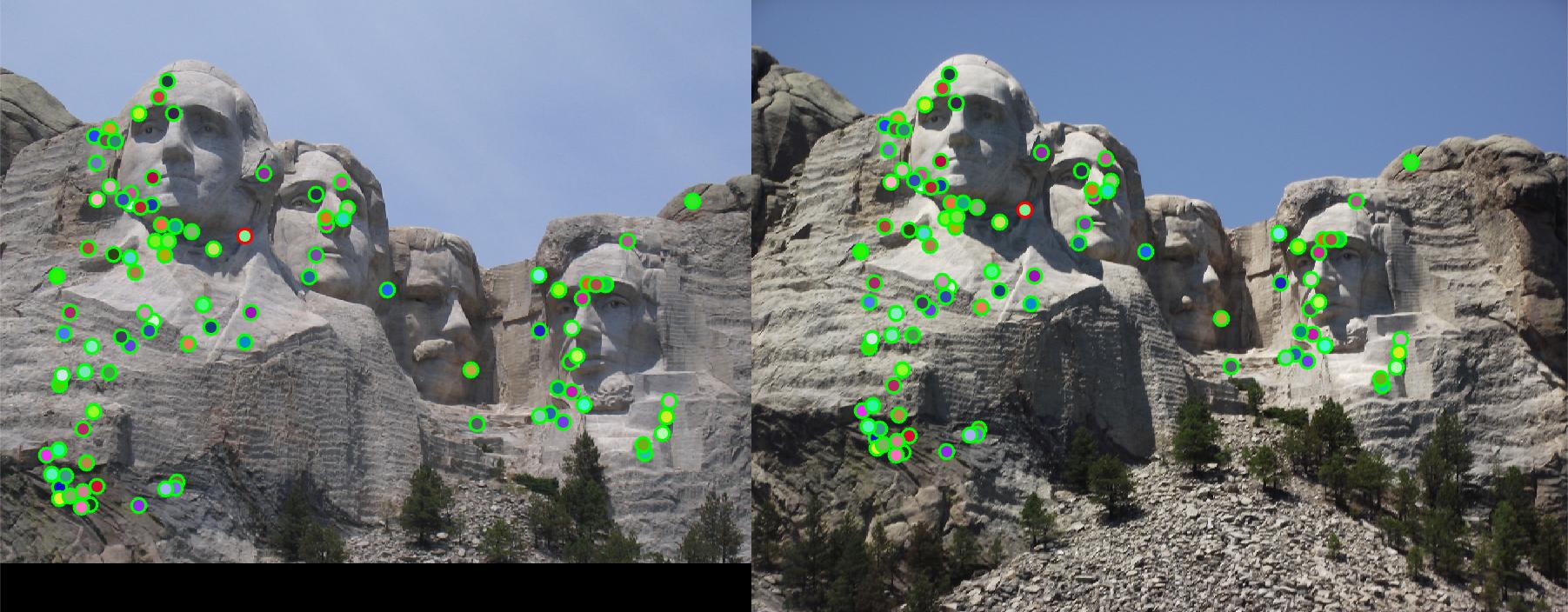
1. Adaptive Non-maximum Suppression (ANMS): 5pts

In case that interest points can be denser in regions of higher contrast, ANMS detect features that are not only local maximum, but also have cornerness score significantly higher (percentage determined by ANMS_diff )than all its neighbors within a radius. Full implementation is in get_interest_point_ANMS.m. Using this ANMS interest point detector and regular baseline feature descriptor, the Mount Rushmore pair get 97% accuracy, which is 5% higher than the regular interest point detector.

copyX = x;
copyY = y;
x = [];y =[];
ANMS_diff = 0.1; 
radius = 0.25*feature_width;
for i = 1:length(copyY)
    local = gray_harris(copyY(i)-radius:copyY(i)+radius,copyX(i)-radius:copyX(i)+radius);
    local = reshape(local,[(radius*2+1)^2,1]);
    current = gray_harris(copyY(i),copyX(i));
    local(local == current) =[];
    if current*(1-ANMS_diff) > max(local)
        x = [x;copyX(i)];
        y = [y;copyY(i)];
    end
end

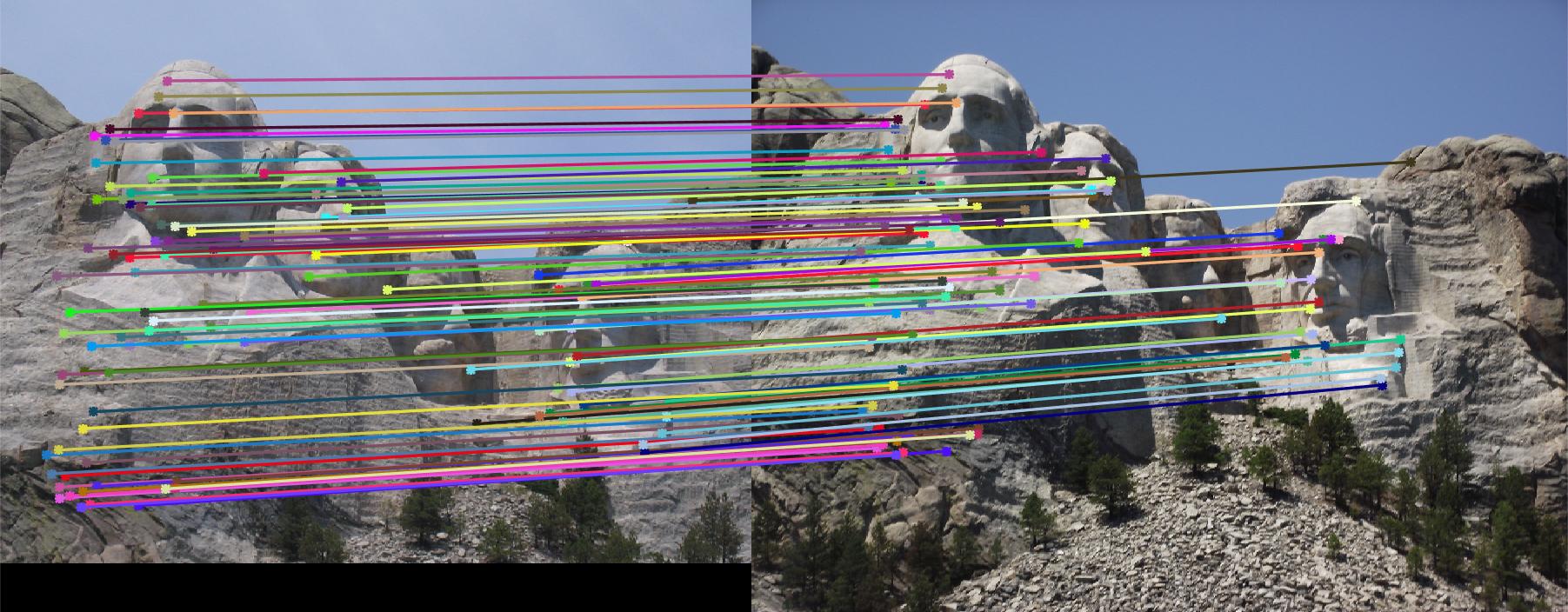
1. Gradient location-orientation histogram (GLOH) spatial layouts: 5pts

GLOH is a variant on SIFT. Instead of using square local sections, GLOH uses log-polar bins to computer orientation histogram. Using radius of 6, 11, 15 to divide regions, get_features_GLOH.m generates 17 sections, each of which has a histogram of 8 bins. The feature size is 17*8. With baseline interst point detector and the GLOH feature extractor, 99% accuracy has been easily achieved on Mount Rushmore pair. The match results are shown in Fig. 7.