Xiaoyu Yuan(xyuan39)

1.Get Interests points

Applying Harris Corner Detection in the following algorithm:

1. Compute the horizontal and vertical derivates of image Ix and Iy by convolving them with derivatives of Gaussians.

Gaussian = fspecial('gaussian', 3, 0.1);
[Gx, Gy] = gradient(Gaussian);
Ix = imfilter(image, Gx);
Iy = imfilter(image, Gy);

2. Compute Ix * Ix, Iy * Iy and Ix * Iy.
3. Convolve the three products with a larger Gaussian.

LargerGaussian = fspecial('gaussian', 9, 1);
Ix2 = imfilter(Ix.*Ix, LargerGaussian);
Iy2 = imfilter(Iy.*Iy, LargerGaussian);
Ixy = imfilter(Ix.*Iy, LargerGaussian);

4. Compute the Harris value by the following equation.

   
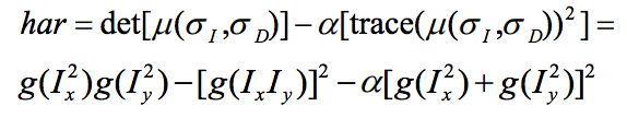
   Harris = Ix2 .* Iy2 - Ixy .^ 2 - k .* (Ix2 + Iy2) .* (Ix2 + Iy2);
   

   Also, in order to prevent index out of bound because of offset from the interests points to its surrounding, I add a border mask to the Harris matrix:

   
   borderMask = zeros(imSize);
   borderMask(1 + feature_width:end - feature_width, 1 + feature_width:end - feature_width) = 1;
   Harris = Harris .* borderMask;
   

5. Find local maxima above a certain threshold and store them as detected interests points.

   
   Threashold = 0.0001;
   k = 0.06;
   threasholdMask = Harris > Threashold;
   connected = bwconncomp(threasholdMask);
   num = connected.NumObjects;
   pixelIdxList = connected.PixelIdxList;
   x = zeros(num, 1);
   y = zeros(num, 1);
   for i = 1:num
       currentInd = pixelIdxList{i};
       currentPix = Harris(currentInd);
       [localmax, maxID] = max(currentPix);
       [j,k] = ind2sub(imSize, currentInd(maxID));
       x(i) = k;
       y(i) = j;
   end
   

2.Get features

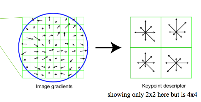
In this step, the local descriptors are returned for those interests points by applying Scale invariant feature transform(SIFT). In my implementation, I construct 4x4 grid cells around the interest points. Then, compute the normalized orientation in 8 directions. Therefore, total of 4 x 4 x 8 = 128 dimensions of descriptors were returned.

features = zeros(length(x), 128);

gaussian = fspecial('gaussian', feature_width, 1);
[Gx, Gy] = gradient(gaussian);

cellSize = feature_width / 4;

Ix = imfilter(image, Gx);
Iy = imfilter(image, Gy);

% calculate orientation of pixels
orientation = atan2(-Iy,Ix)*180/pi;
magnitute = sqrt(Ix .* Ix + Iy .* Iy);

reduce_g = fspecial('gaussian', feature_width, feature_width/2);
for i = 1:length(x)
    currentX = x(i) - 2*cellSize;
    for j = 1:4
        currentY = y(i) - 2*cellSize;
        for s = 1:4
            currentCell = orientation(currentY:(currentY + cellSize - 1), currentX:(currentX + cellSize - 1));
            currentMag = magnitute(currentY:(currentY + cellSize - 1), currentX:(currentX + cellSize - 1));
            currentMag = imfilter(currentMag, reduce_g);
                for k = -4:1:3
                    mask = currentCell >= k*45 & currentCell < (k+1)*45;
                    mag_masked = currentMag(mask);
                    histo = nnz(mag_masked);
                    features(i, (j - 1) * 32 + (s - 1) * 8 + k + 5) = histo;
                end
            currentY = currentY + cellSize;
        end
        currentX = currentX + cellSize;
    end
    total = sum(features(i,:));
    features(i, :) = features(i, :)/total;
end
end

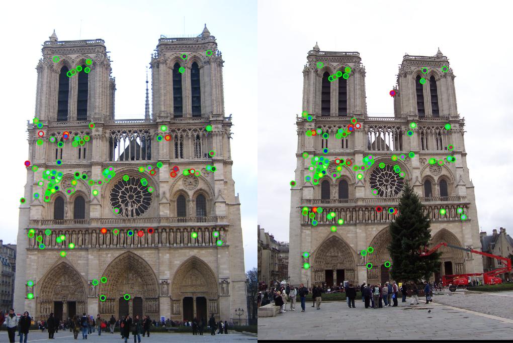
	detected features of Notre Dame with threshold = 0.0001 and alpha = 0.04
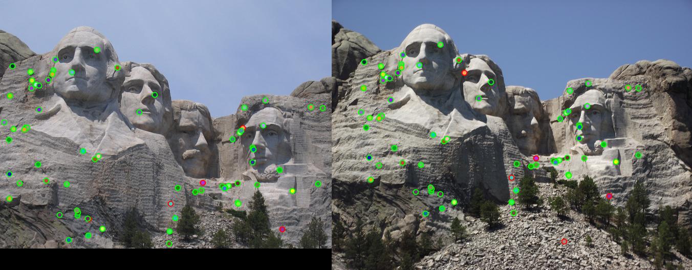
	detected features of Mount Rushmore with threshold = 0.0001 and alpha = 0.04
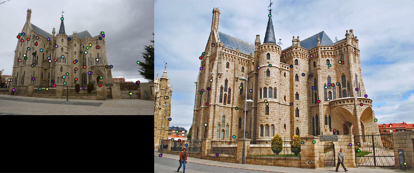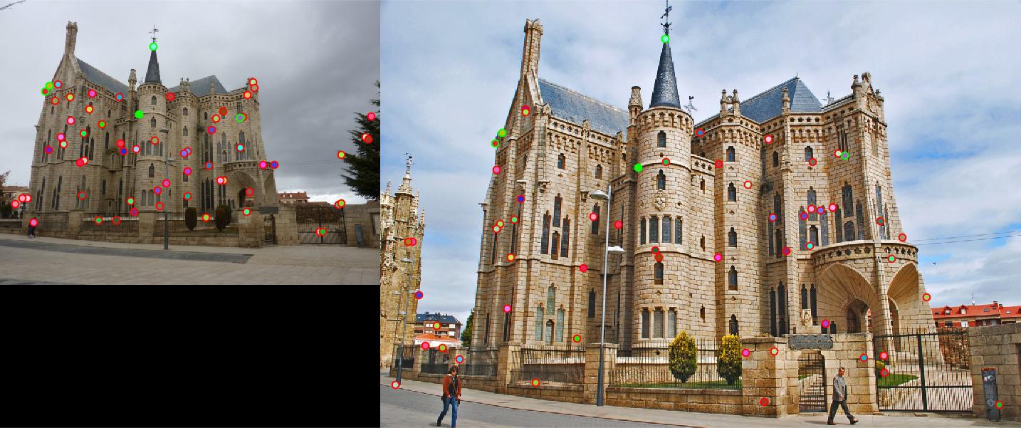
	detected features of Episcopal Gaudi with threshold = 0.0001 and alpha = 0.06

3.Features matching

The thirs step is the matching of two images. For each descriptor in feature 1, calculate the distance between it and every descriptor in feature 2. Then, store all the results and sort the final array. Apply the nearest neighbout distance ratio to select the preferable matching points. The ratio is defined by the difference between the smallest distance between two descriptors in each features divided by the second smallest distance between other two. Finally, a threshold is set for choosing fitted points, in this case, 0.85

threshold = 0.85;
confidences = [];
matches = [];
k = 1;
for i = 1 : size(features1, 1)
    for j = 1: size(features2, 1)
        currentDist(j, :) = sum((features1(i,:) - features2(j,:)).^2);
    end
    [currentDist, indexlist] = sort(currentDist);
    ratio = currentDist(1)/currentDist(2);
    if ratio < threshold
        matches(k, 1) = i;
        matches(k, 2) = indexlist(1);
        confidences(k) = ratio * 100;
        k = k+1;
    end
end
	

The ratio is stored for evaluation of the resulting image matching.

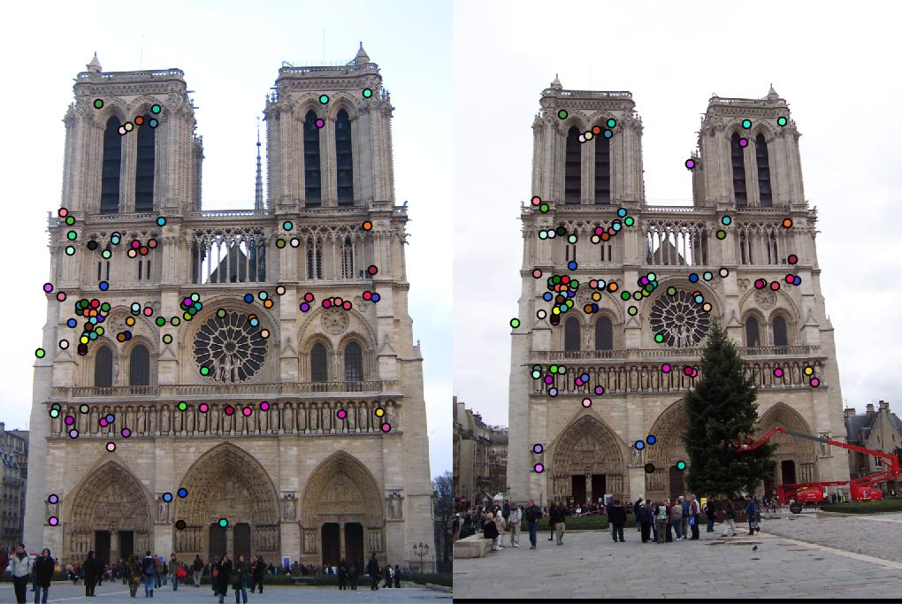
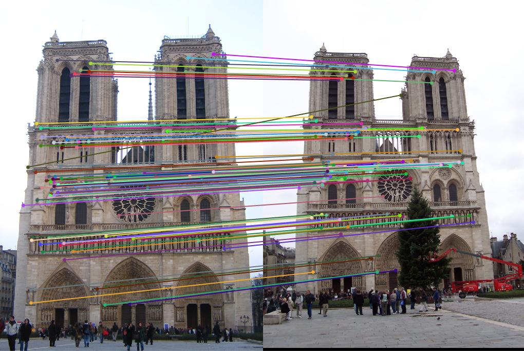
Notre Dame: threshold : 0.6	Result: 95 total good matches, 12 total bad matches. 89% accuracy
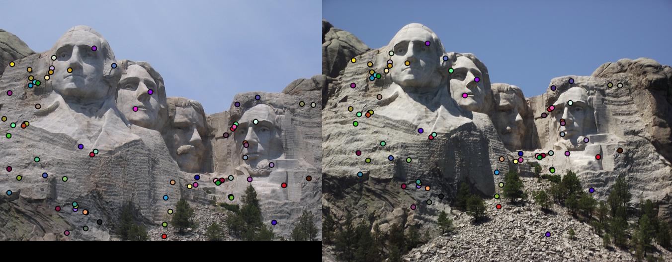
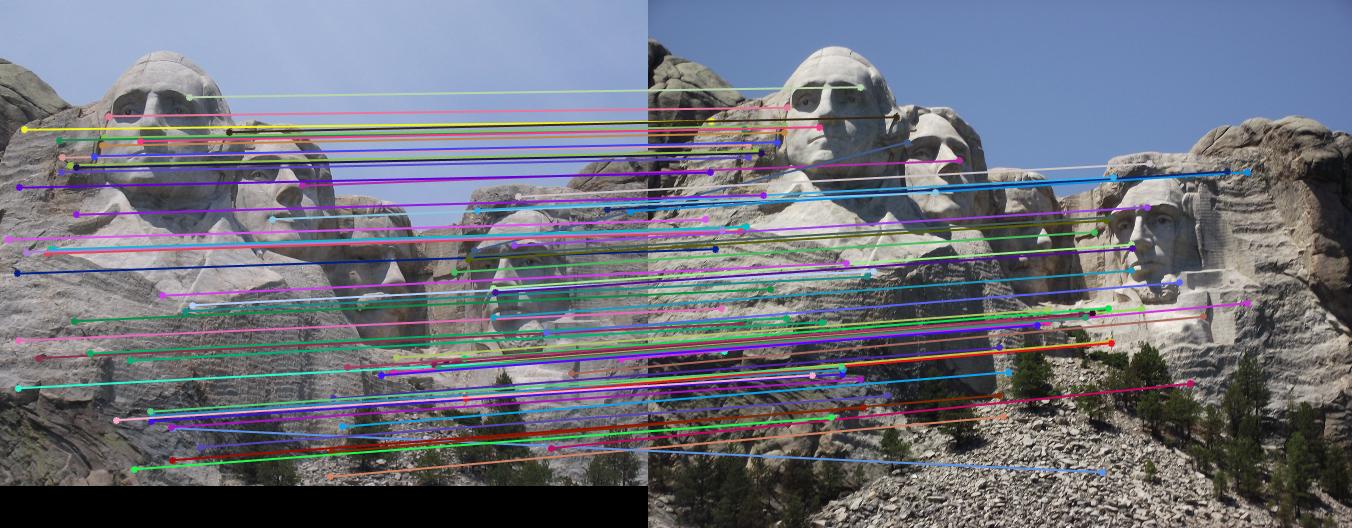
Mount Rushmore: threshold : 0.6	Result: 68 total good matches, 5 total bad matches. 93% accuracy
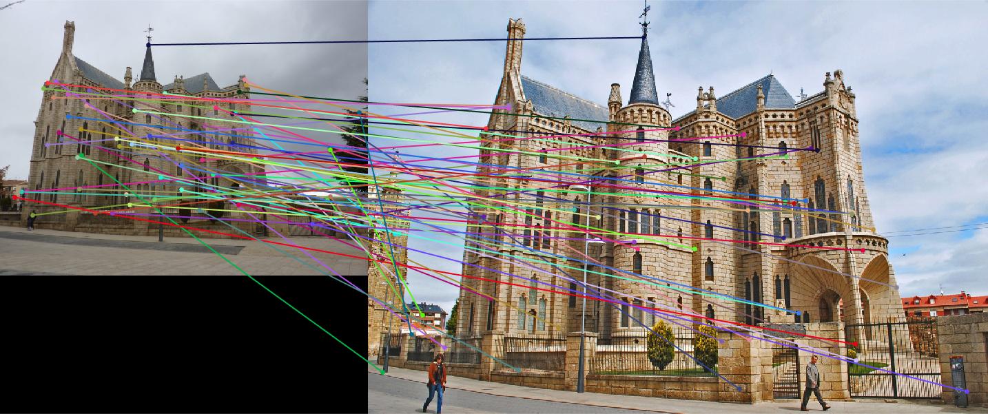
Episcopal Gaudi: threshold : 0.85	Result: 5 total good matches, 59 total bad matches. 8% accuracy

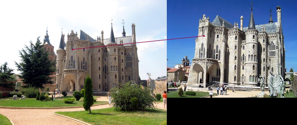
4.Other examples

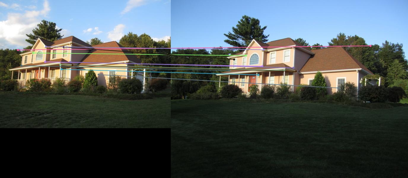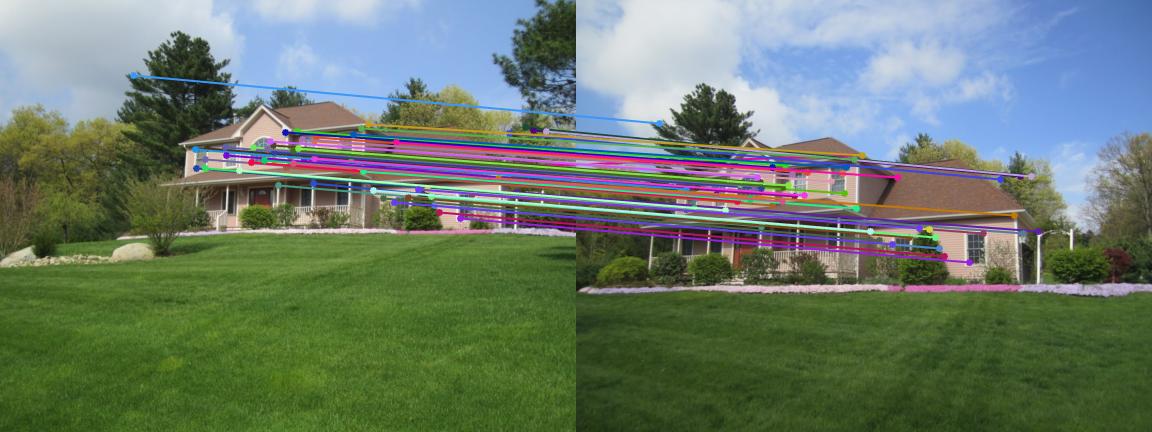
Example1	Example2
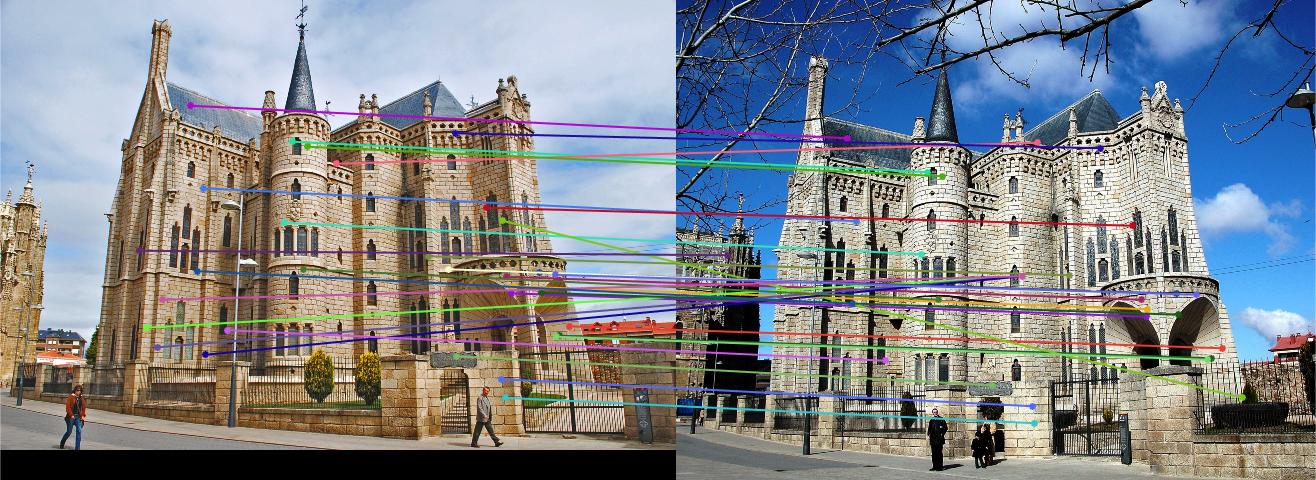Example3	Example4