Project 2: Local Feature Matching
The goal of this assignment is to create a local feature matching algorithm using a simplified version of the famous SIFT pipeline. There are following steps to implement this algorithm:
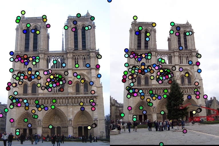
- Implement the Harris corner detector to get interesting points.
- Generate feature descriptors from interesting points using a SIFT-like method.
- Utilize nearest neighbor distance ratio test to match features.
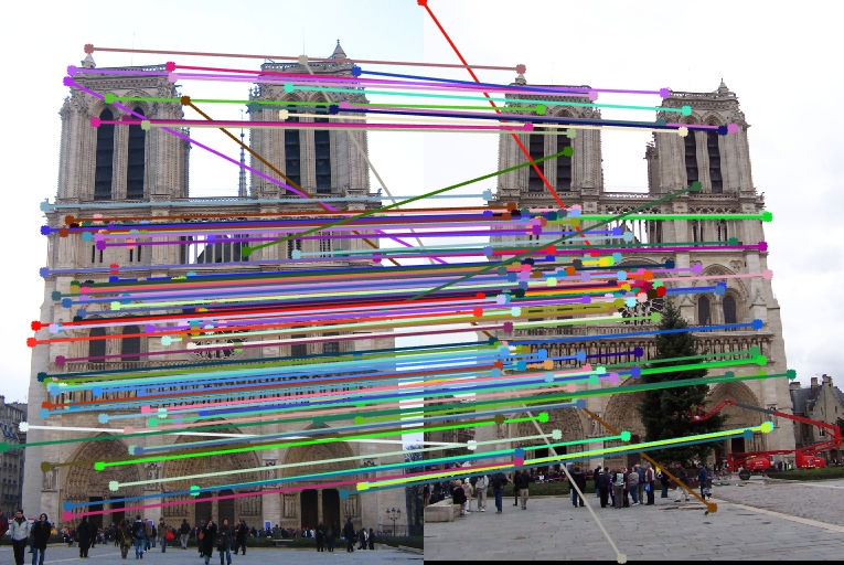
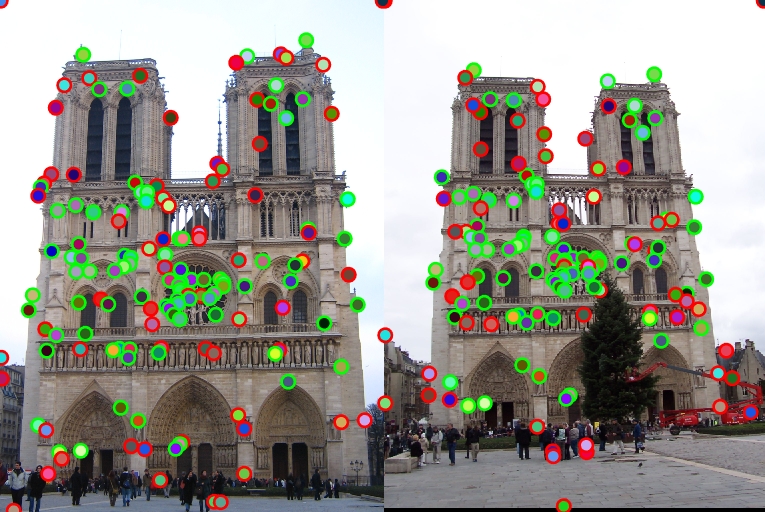
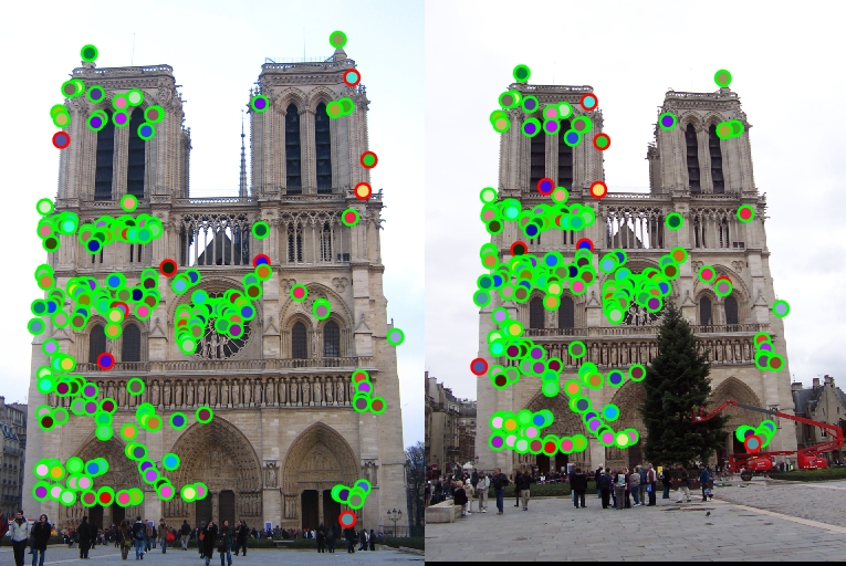
The following pictures are the result on the Notre Dame pair. It has 88% accuracy, with 141 total good matches and 20 total bad matches.
|
1. Interest point detection (get_interest_points.m)
This part uses the Harris corner detector to detect corners as interesting points.
First of all, we blur the image using a Gaussian filter with the standard deviation of 1 and size (6, 6). After that, we set dx = [-1 0 1;-1 0 1;-1 0 1], dy = the transpose of dx. Compute the horizontal and vertical derivatives of the image Ix and Iy by convolving the image with dx and dy. Then the auto-correlation matrix A can be written as
$$\huge A = \omega * \left[ \begin{matrix} I_x^2 & I_xI_y \\ I_xI_y & I_y^2 \end{matrix} \right]$$
where w is a Gaussian filter with the standard deviation of 2 and size (7, 7).
After computing A, we can get a matrix of harmonic mean as
$$\huge R = \frac{det A}{tr A} = \frac{\lambda_0\lambda_1}{\lambda_0+\lambda_1}$$
We find the biggest value Rm in this matrix. If R(i, j) > 0.01*Rm, point (i, j) is selected.
A simple way of non-maximum suppression is implemented to get better results. For each interesting point, we look at the neighboring window with radius 3, if it indeed has the maximum value then it is preserved.
2. Local feature description (get_features.m)
We implement a SIFT-like local feature description to describe interesting points. The following picture briefly illustrates the idea of this part.
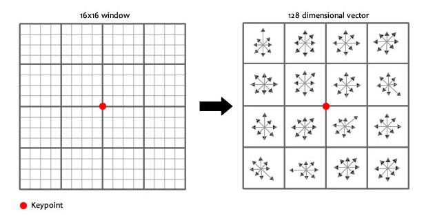
A feature of 4*4*8 is computed when the width of window equals 16, as the picture shown. For a window size of feature_width, a (feature_width* feature_width/2) dimension vector is computed from each interesting points.
To compute feature descriptions, we first compute the horizontal and vertical derivatives of the image Ix and Iy. Then we loop through all interesting points, find the patch of Ix and Iy of size (feature_width, feature_width) and convolve them with a Gaussian filter. After that, the scale and orientation of this point can be computed by
$$\huge S(P) = \sqrt{I_x^2(P)+I_y^2(P)},O(P) = arctan\frac{I_y(P)}{I_x(P)}$$
A gradient orientation histogram is then computed in each subregion. Finally, we combine these gradient orientation histograms together to get an n* (feature dimensionality) array of features, where n is the number of interesting points.
3. Feature matching (match_features.m)
With feature vectors, we can compute the distance between any two interesting points. For each points in image1, we compute the dot product between the corresponding row of descriptor and the transpose of the feature matrix of image2. Then we sort the arccos value of the dot product to get an array val. The nearest neighbor distance ratio can be computed as
$$\huge NNDR = \frac{d_1}{d_2} = \frac{val_1}{val_2}$$
We choose 0.7 as the threshold, which means a points is selected when NNDR < 0.7. Intuitively, the less the threshold is, the higher the accuracy is. However, if the threshold is small, we can get only a few points.
4. Test Results
The result on the Notre Dame pair with distance ratio of 0.7 and features having width of i6 pixels has 88% accuracy, with 141 total good matches and 20 total bad matches.
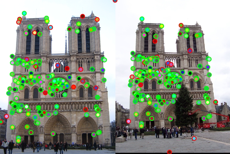
When change feature width to 8, the accuracy quckly drops down to 0.57. When change feature width to 32, the accuracy rises to 0.96 with 196 total good matches and 9 total bad matches. However, it needs more time to compute the result. The left picture is for the feature of width 8 and the right is for the width of 32.
|
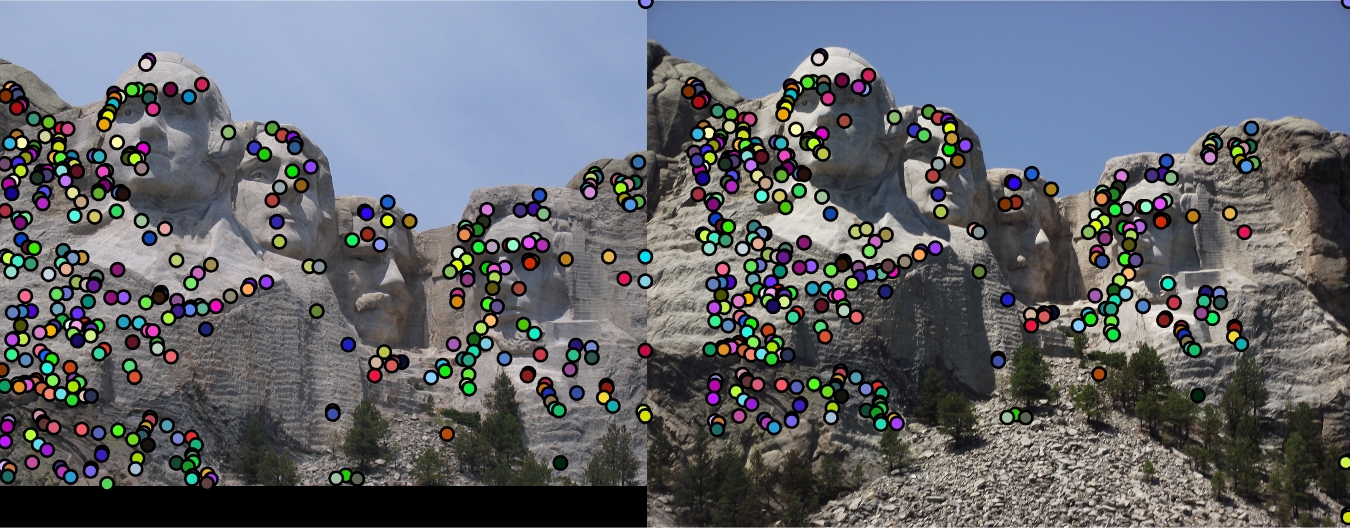
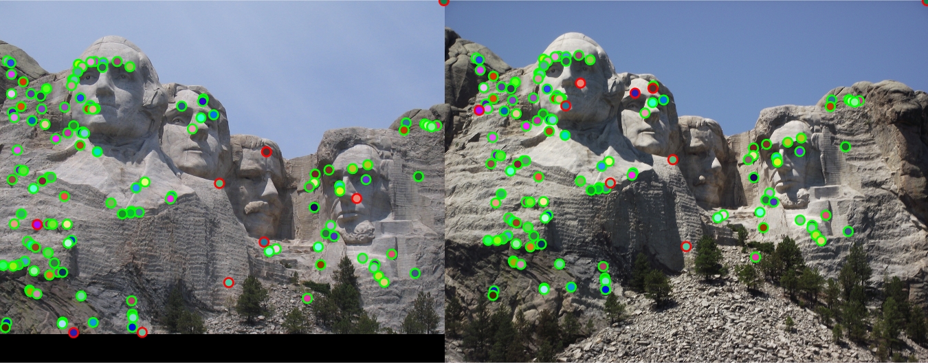
The result on the Mount Rushmore pair with distance ratio of 0.7 and features having width of i6 pixels has 93% accuracy, with 363 total good matches and 26 total bad matches.
|
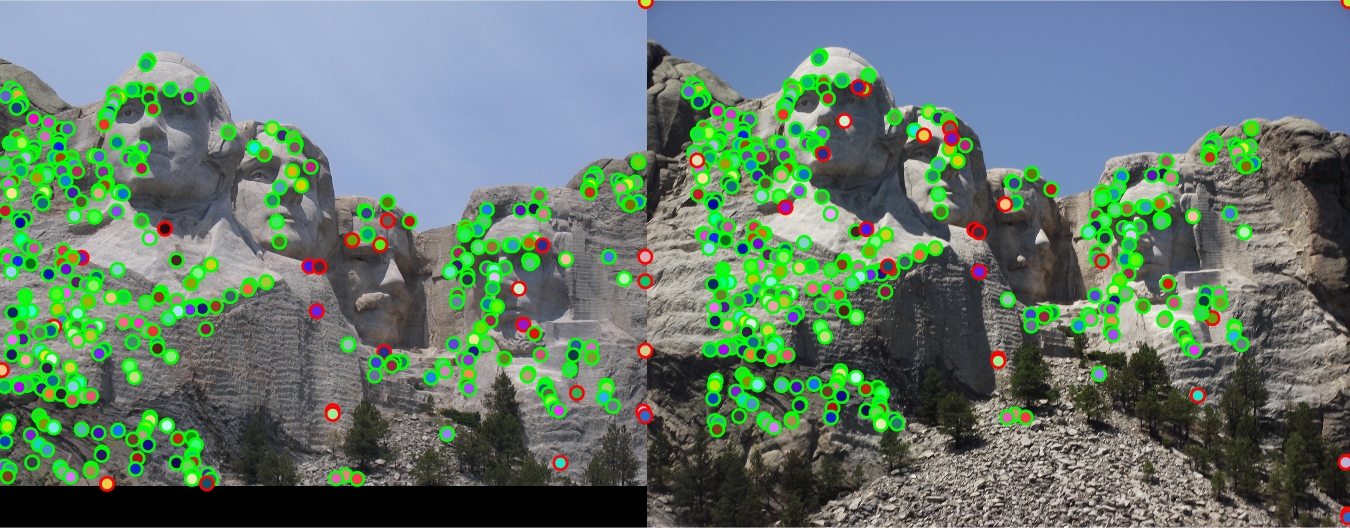
Keep the feature width as 16, when the distance ratio equals 0.6, the Mount Rushmore pair has 129 total good matches, 9 total bad matches. The accuracy doesn't change when reducing the ratio from 0.7 to 0.6 for this pair. The reason may be that the error points are very close to correct points so we can't fix the problem by reducing the distance ratio.
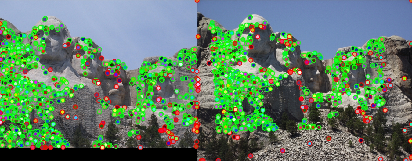
When increasing the distance ratio to 0.8, the Mount Rushmore pair has 87% accuracy, with 737 total good matches and 113 total bad matches. The number of points increase quickly and the match accuracy drops down.
The left picture is for the ratio of 0.6 and the right is for the ratio of 0.8.
|
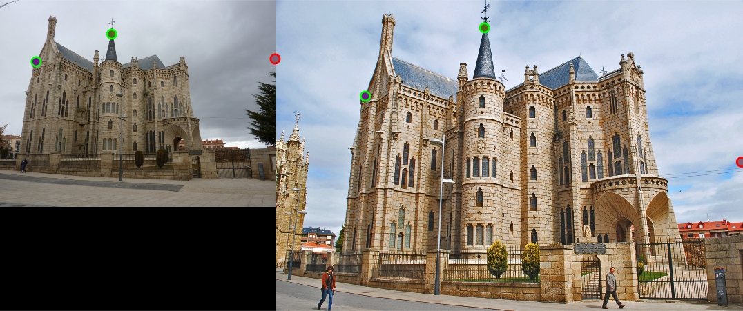
The result on the Episcopal Gaudi pair with distance ratio of 0.7 and features having width of 32 pixels has 67% accuracy, with 2 total good matches and 1 total bad matches. My algorithm doesn't work well with this pair of pictures.

|