Project 2: Local Feature Matching
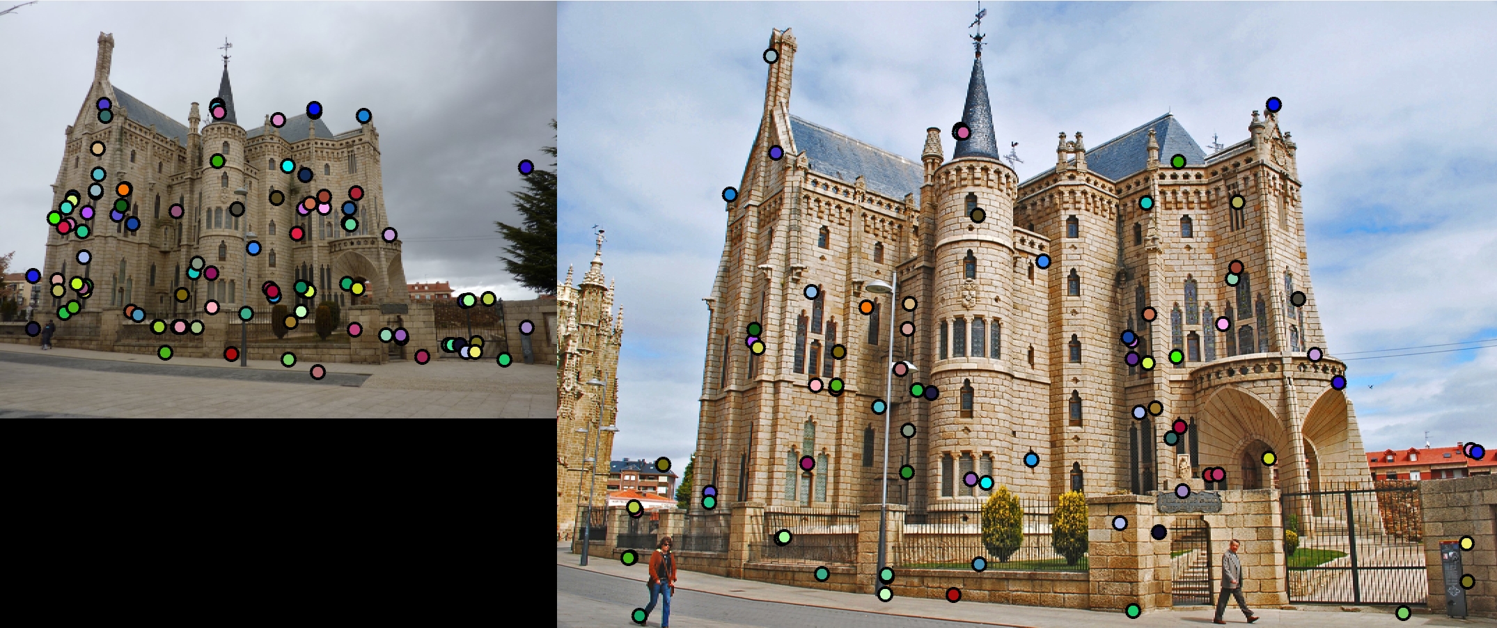
Episcopal Gaudi interest points.
Task 1: get_interest_point.m
The project is divided into 3 functions. The first one is to find interest points. The specific steps are as follows:
- Blur the image with a standard gaussian to remove noise.
- Get Ix and Iy by implementing imgradientxy function
- Calculate Ixx = Ix^2, Iyy = Iy^2 and Ixy=Ix .* Iy and convolve them with a larger gaussian.
- Calculate R = det(M)-alpha*trace(M)^2 = (ix^2)*(iy^2) - (ix*iy)^2 - alpha*(ix^2+iy^2)^2 for every pixel.
- Set up threshold and construct a binary map to indicate pixels above the threshold value, select local maximum by using bwconncomp built-in function.
- Translate the x,y coordinate of local maximum and set them as coordinates for interest points
Task 2: get_features.m
The second tasks asks us to describe the feature around interest points. SIFT is implemented as the following:
- Use a small Gaussian filter to blur the image.
- Generate matrices of maginute and gradient of the image using imgradient.
- For each interest point, patch it up with a feature_width X feature_width(16x16) window.
- Divide the window into 16 4x4 cells.
- For each pixel in the patch, categorize the direction of the gradient into one of the 8 bin, and add the magnitue of the gradient to the histogram corresponding to that orientation.
- Linearize the histograms into a 1x128 vector as feature description.
- Normalize the vector and and append feature into feature list
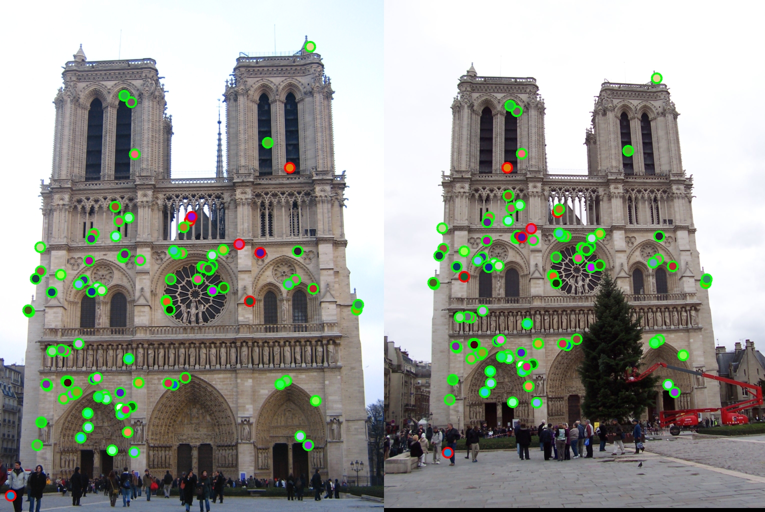
Initially when doing the normalized patch as feature descriptions, the accuracy jumped from nearly 0% to 42%. When SIFT-life feature is implemented, the accuracy rose up to 66% for Notre Dame pair.
Task 3: match_features.m
In Tast 3, we are supposed to match the features of two similar images.
- Iterate through features in feature_1 list and find nearest and second nearest features from feature_2 list.
- Implement the ratio test.
- Since we want the feature to be near corresponding feature and away from other features, we use D2/D1 as confidence indication
- Sort the confidence in descending order so most confident matches are at the top
- The following part is my code for this task
Code for match_features.m
num_features = min(size(features1, 1), size(features2,1));
matches = zeros(num_features,2);
confidences = zeros(num_features,1);
for i = 1:size(features1,1)
    shortest = Inf;
    second_shortest = Inf;
    nearest = 0;
    for j = 1:size(features2,1)
        distance = norm (features1(i,:) - features2(j,:));
        if distance < shortest
            shortest = distance;
            nearest = j;
        elseif distance < second_shortest
            second_shortest = distance;
        end
    end
    matches(i,:) = [i nearest];
    confidences(i) = second_shortest / shortest;
end

% Sort the matches so that the most confident onces are at the top of the
% list. You should probably not delete this, so that the evaluation
% functions can be run on the top matches easily.
[confidences, ind] = sort(confidences, 'descend');
matches = matches(ind,:);
Results in a table
|
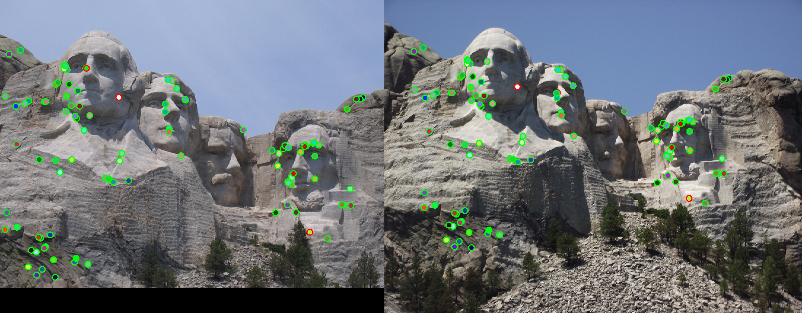
The final accuracy rate I achieved was 93% on Notra Dame pairs and 97% on Mount Rushmore pairs. Unfortunately the Episcopal Gaudi pair is low as 4%(tuning the alpha and threshold value doesn't seem to affect accuracy significantly). I think finding local maximum is a very tricky part in this project. Using bwconncomp to group binary map regions is a very interesting way of tackling the problem. Another thing I observed through this homework is that the larger gaussian filter in get_interest_poins.m played a huge role in terms of accuracy. When I first use the default setting of the sd value in the filter, it's too big and it actually elimantes all the useful corner information I need to find corret interest points. After many hours of debugging and trying did I finally realize it's this parameter value affecting the performance of the function and changed it to 0.1