Project 2: Local Feature Matching
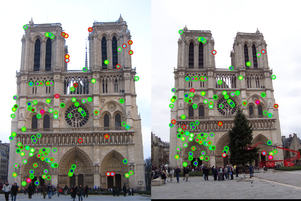 |
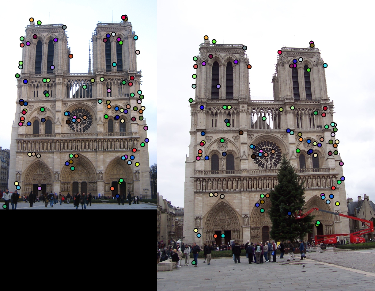
| Keypoint matches for Notre Dame |
The objective of the project Local Feature Matching is to extract interest points from two images and match the key point with a local feature descriptor. The project would serve well for matching the multiple views of the same physical scene.
An output of the project is shown above. Two views of Notre Dame are presented with interest points marked. The green points represent correct matching while the red ones correspond to the incorrect ones. The image shows the top 100 matches in terms of confidence. Implemented by the basic methodology, among the top 100 matches presented, 83 were correct matches, achieving the accuracy of over 80%.
Methodology
The program implementation includes finding interest points, getting local feature descriptor and matching features. The Methodology section will cover each of them.
1. Find Interest Points
The first method used in finding the interest points is similar to the Harris corner detector. Each pixel is assigned a score based on their gradients in x and y direction. The interest points are selected based on the score they obtained. A threshold is set to ensure that the points are indeed interest points.
Non-maxima suppression is used in this process to eliminate the neighbor points of the interest points. Only the pixel with the maximum score within a window is selected. The code for suppression is shown as follows:
max_local_score=colfilt(score, [feature_width, feature_width], 'sliding', @max);

score_suppressed=score.*(score==max_local_score);
 |
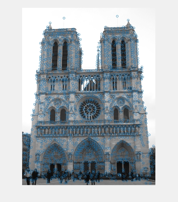 |
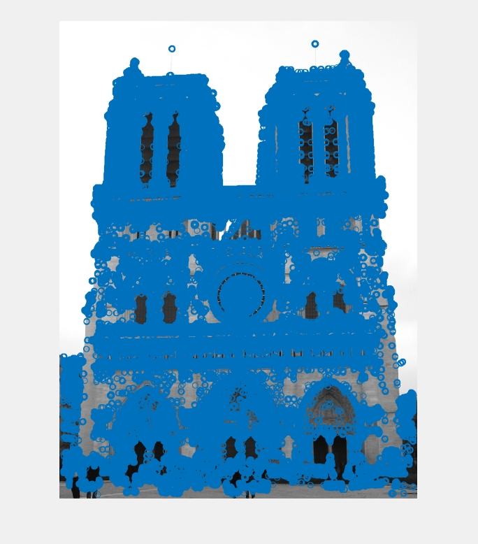
| Without Suppression | With Suppression |
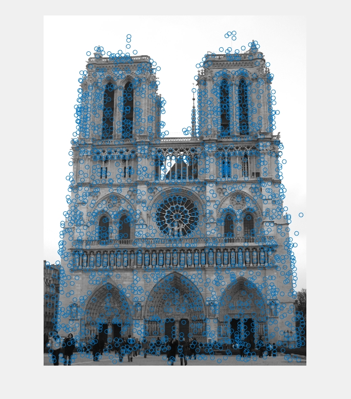
The left image above is the result without suppression. It contains many more points, which are actually not interest points, compared to the right one.
2. Calculating Local Features
To obtain the feature vector of each interest point, the program implements the following thing.
1. Acquire a window around the point. Size configured by the parameter featuer_width.
2. Partition the window into 16(=4*4) cells.
3. Apply the derivative operator in different directions to the window and gaussian-filter it.
4. Calculate the sum of derivative in each direction for each cell(8 directions by default, 45 degree between consecutive ones).
5. Use the result 8*16=128 vector as the feature.
3. Matching Features
For each feature, the function finds the nearest neighbor and the second nearest neighbor in the other image. If the ratio of the distances ( d(feature, nearest neighbor)/ d(feature, second nearest neighbor) )is below a threshold, the feature and its nearest neighbor is recognized as a match with confidence=1/ratio. The threshold is set to 0.7.
Extra Points Implementation
Several extensions are implemented in the project to obtain additional conclusions and improve the performance.
1. SIFT Parameter Tuning
Parameters are changed to test their impact on the performance.
The following table shows the result of tuning the number of cells and the number of orientations contained by the
feature vector. The following conclusions can be drawsn:
1. Manipulating the number of cells can have a huge impact on the performance. 16 (4*4) cells would give the best result
compared to the other 2 cases. While a smaller number of cells would find more matches, most of them are incorrect. A
larger number of cells give decent accuracy but meanwhile fewer matched feature points.
2. The number of orientations used to represent the histogram does not have a huge impact the performance. As long as the
histogram is represented by more than a proper number of directions (in this case, 4 orientations are enough) the
performance would be fine. However, more orientations result in more computation and therefore longer response time.
| #Cells | #Orientations | Top 100 Accuracy | Total Accuracy | Total Matches |
| 4=2*2 | 360/30=12 | 54% | 39% | 216 |
| 4=2*2 | 360/45=8 | 51% | 41% | 211 |
| 4=2*2 | 360/60=6 | 54% | 39% | 216 |
| 4=2*2 | 360/90=4 | 52% | 39% | 224 |
| 16=4*4 | 360/30=12 | 83% | 74% | 141 |
| 16=4*4 | 360/45=8 | 83% | 74% | 138 |
| 16=4*4 | 360/60=6 | 83% | 74% | 139 |
| 16=4*4 | 360/90=4 | 82% | 73% | 141 |
| 64=8*8 | 360/30=12 | 75% | 75% | 101 |
| 64=8*8 | 360/45=8 | 76% | 75% | 101 |
| 64=8*8 | 360/60=6 | 76% | 75% | 106 |
| 64=8*8 | 360/90=4 | 75% | 75% | 97 |
The following table shows the result of tuning the size of feature. The performance degrades as the size increases from 16. A possible explanation is that the feature contained by the image is around exactly 16 so it gives the best performance.
| Feature Size | #Cells | #Orientations | Top 100 Accuracy | Total Accuracy | Total Matches |
| 8 | 16=4*4 | 360/45=8 | 80% | 68% | 220 |
| 16 | 16=4*4 | 360/45=8 | 83% | 74% | 138 |
| 24 | 16=4*4 | 360/45=8 | 73% | 73% | 73 |
| 32 | 16=4*4 | 360/45=8 | 66% | 66% | 47 |
2. DoG feature extraction in different scales
The algorithm is in Szeliski Page 217 and illustrated with
Figure 4.11. Basically the image is constantly gaussianed with growing standard deviation. The two images at neighboring standard
deviation is subtracted to obtain the difference image. At least 3 difference images are needed. A point is an interest point if it
is the local maxima/minima (3*3 window) in the middle image and its value in the middle image is still the largest/smallest compared to the 3*3 window
in the upper and lower image. In other words, a point needs to beat other 26 values to be recognized as an interest point.
Afterwards, the image is scaled down and applied the same algorithm upon to find features of larger size.
The following figure can illustrate the algorithm better.
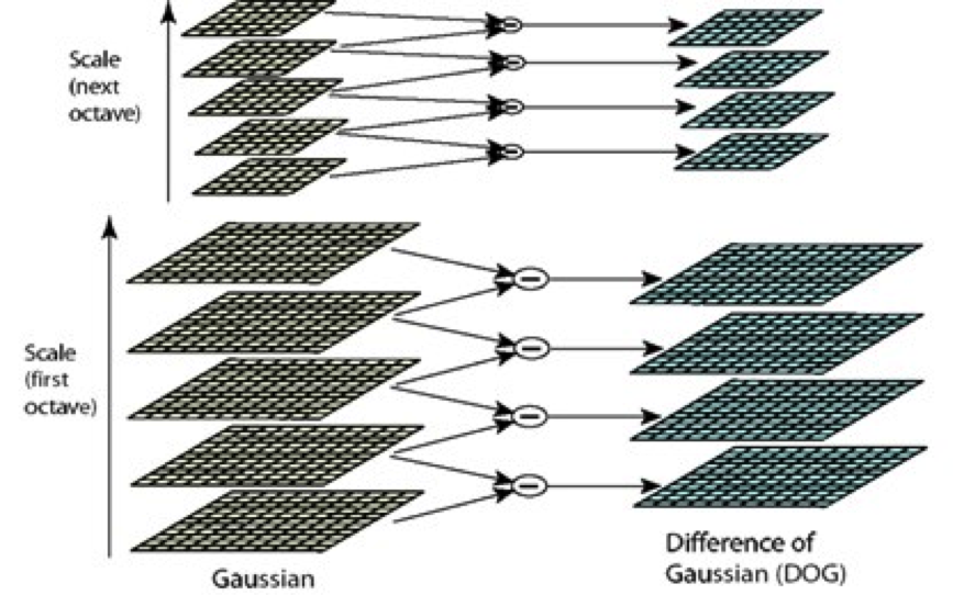 |
| Implementation of the scale invariant interest point extraction. Source: http://gpgpucolumbia2015imasweebly.com/images/dog.png |
Below is my implementation of the algorithm.
    image1=imgaussfilt(image, sigma);
    image2=imgaussfilt(image, sigma*k);
    image3=imgaussfilt(image, sigma*k^2);
    image4=imgaussfilt(image, sigma*k^3);

    diff1=image1-image2;
    diff2=image2-image3;
    diff3=image3-image4;

    max_diff1=colfilt(diff1, [3 3], 'sliding', @max);
    max_diff2=colfilt(diff2, [3 3], 'sliding', @max);
    max_diff3=colfilt(diff3, [3 3], 'sliding', @max);

    max_point=max(max_diff1, max_diff3);
    max_diff2=max(max_point, max_diff2);
    max_diff2=(max_diff2==diff2).*diff2;

    [y, x]=find(max_diff2>threshold);
The following plots the interst points obtained by this algorithm. It has a decent result with most of the important points obtained.
 |
|
| Scale Invariant Features | Original Algorithm |
3. Feature extraction according to the scale
In accordance with the implementation of the second extra point, the feature are obtained in a different way. When the interest point is not in the original scale of the image, the image is scaled down according to the corresponding scale parameter.
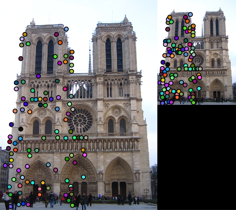 |
| Scale Invariant Match (Only partially shown here, the rest are similar. The whole match will give a messy image and cannot be visualized properly) |
 |
| Original Algorithm |
I have tried to scale down one of the image and compare the small image to the original image itself. The algorithm can definitely extract the matches with 100% accuracy, while my original algorithm without scale invariant features failed.
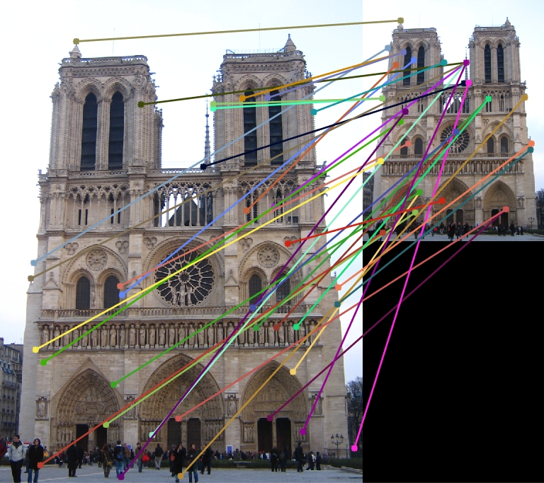
 |
When trying to scale down one of the image and compare it to the other view, I still obtained acceptable performance. Some matches are found while some others are incorrect matches. If the scale factor is set to exactly represent the scale difference of the two views, higher accuracy can be expected. Anyways, the accuracy is still decent, compared to the basic algorithm.
Results Display
|
| Notre Dame (83% Accuracy) |
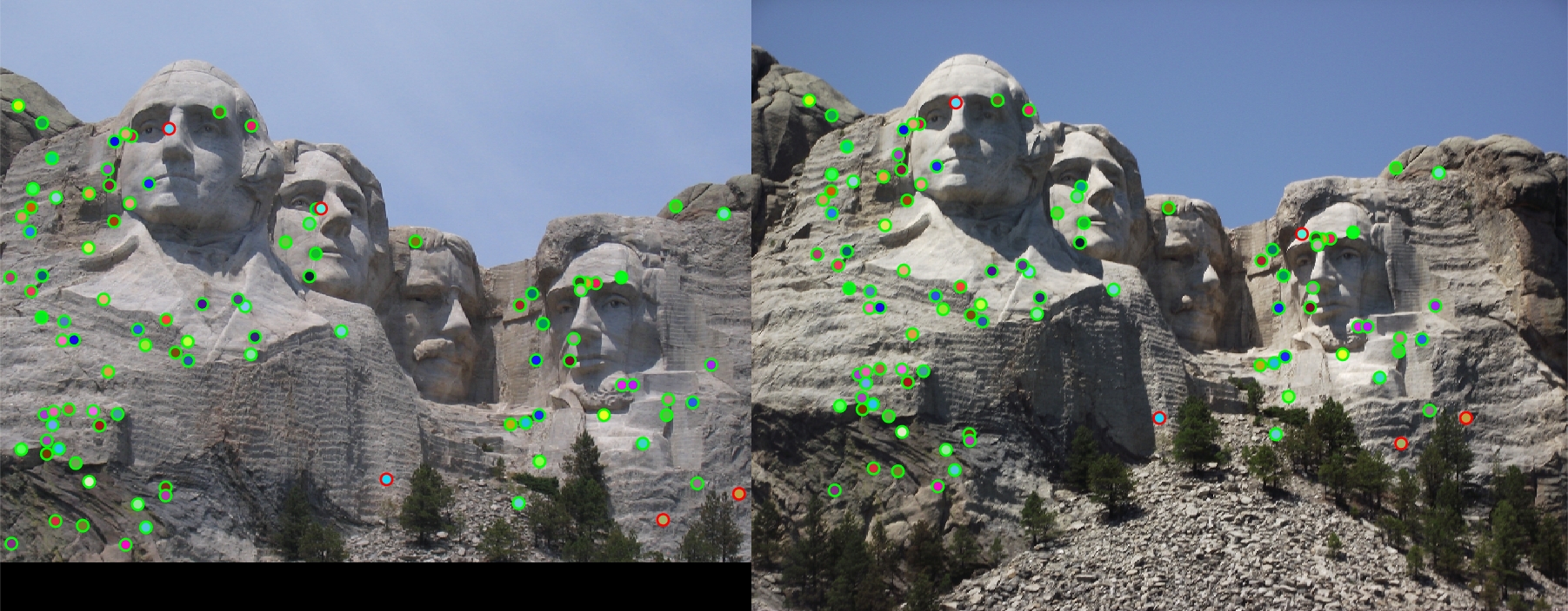 |
| Mount Rushmore (95% Accuracy) |
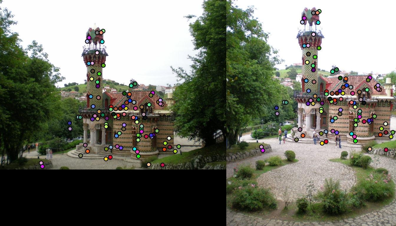 |
| Capricho Gaudi |
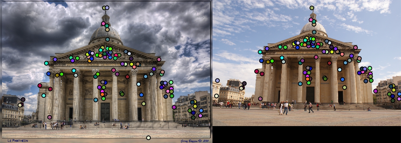 |
| Pantheon Paris |