Project 2: Local Feature Matching
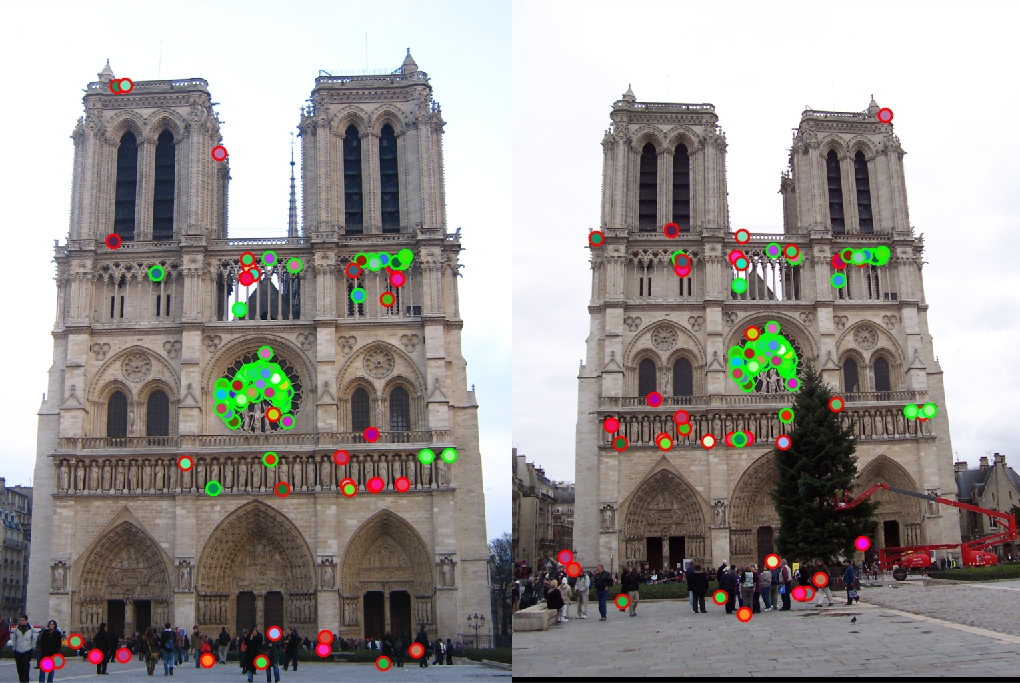
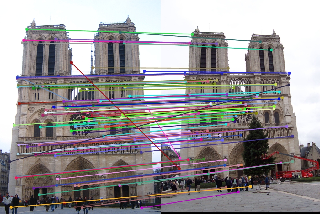
Two images of Notre Dame with matched interest points
Project two involved finding interest points in two similar images and then finding matches that correspond to the same spatial position in both images. This process was divided into three steps:
- Getting interest points
- Describing the local features
- Matching the features
Different approaches and thresholds were tested in each of the steps, with the goal of trying to maximize the number of correct matches per image pair.
Finding Interest Points
Interest points were determined by finding Harris corners. The Harris response was calculated as follows:
	xgrad = imfilter(blurred, [-1 0 1],'symmetric');
	ygrad = imfilter(blurred, [-1;0;1],'symmetric');

	Ix2 = imgaussfilt(xgrad.^2, 2, 'FilterSize', 3);
	Ixy = imgaussfilt(xgrad.*ygrad, 2, 'FilterSize', 3);
	Iy2 = imgaussfilt(ygrad.^2, 2, 'FilterSize', 3);

	R = (Ix2.*Iy2 - Ixy.^2) - k*(Ix2 + Iy2).^2;
The response matrix was then dilated to make the maximal values propagate to its neighbors. Then a threshold was used to filter responses that were a certain amount smaller than the maximal response detected. An edge mask was also used to get rid of interest points that were too close to the edge. The coordinates where the original response value was equal to the dilated response value was chosen as an interest point, since the two being equal means that it is a local maximum.
Getting Local Feature Descriptions
At first, normalized patches were used. This involved taking a 16x16 region around the keypoint, and then using the brightness values of each pixel in that region to form a descriptor. The descriptor was then normalized to have a sum of 1. A SIFT-like feature was also used to describe each keypoint. A square region around the keypoint with a predetermined feature width was first extracted. Then, the X and Y gradients were once again calculated. The distance and direction of each pixel's gradient was calculated as follows:
	dist = sqrt(xgrad.^2 + ygrad.^2);
	directions = atan2(ygrad, xgrad);
Matching Features
Matching a feature from one image to another simply involved taking a descriptor from the first image and then finding the closest descriptor from the second image.
The first and second images were then swapped to make sure that the closest match to the descriptor chosen from the second image was the descriptor from the first image.
If this did not hold, the match was discarded.
The ratio test was also implemented. This involved finding the ratio between the distance of a keypoint and its closest match, and the distance of it and its second closest match.
Matches with a ratio of more than 0.7 were discarded to avoid using ambiguous keypoints and therefore finding wrong matches.
Results
Initial Results
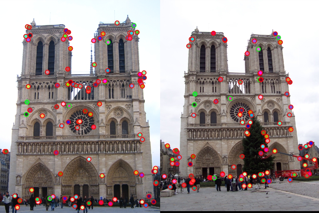
The Notre Dame image pair was used to see how changes to the process affect match accuracy. At first, the descriptor used for each keypoint was its normalized patch. The ratio test was not used to filter out ambiguous points.
|
This resulted in an accuracy of 64% when looking at the 100 most confident matches.
Switching to SIFT Descriptors
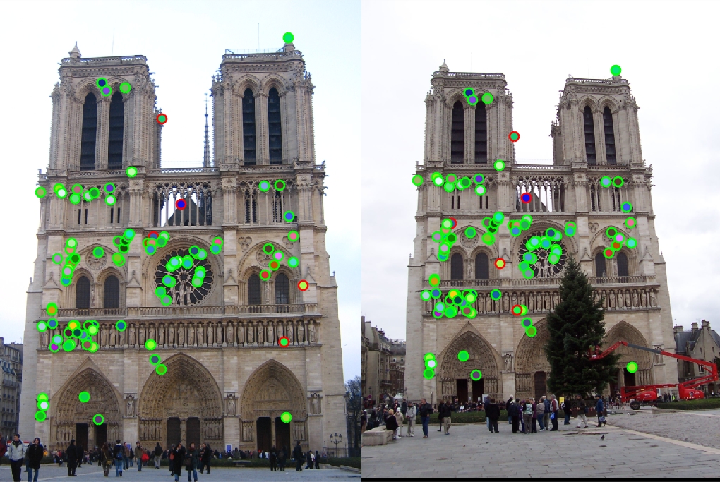
The descriptor used was then switched from normalized to patches to a SIFT-like descriptor. The ratio test was still not implemented at this point.
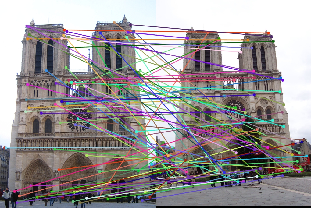
|
This time, only a 7% match accuracy was seen. This is due to the SIFT-like descriptor being more abstract than a normalized patch in regards to the actual pixel values of the image. Therefore, it is more difficult to match up keypoints than when using normalized patches, since there is less data about the actual image. Further work has to be done to throw out ambiguous matches, even though their distance may be very small.
Adding the Ratio Test
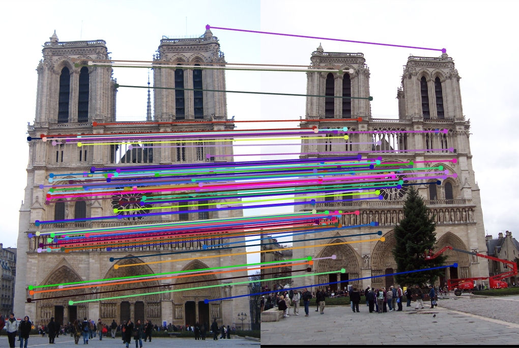
Next, the ratio test was added to discard any matches that are determined to be too ambiguous and therefore have a high chance of being incorrect.
|
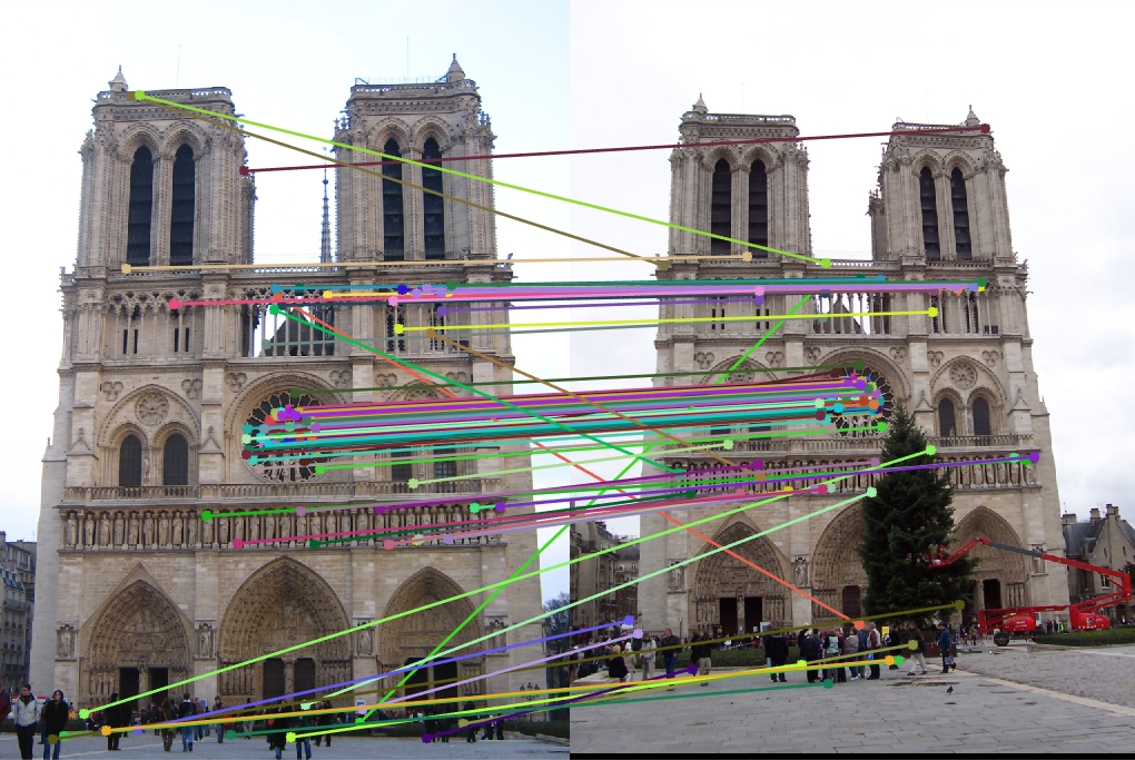
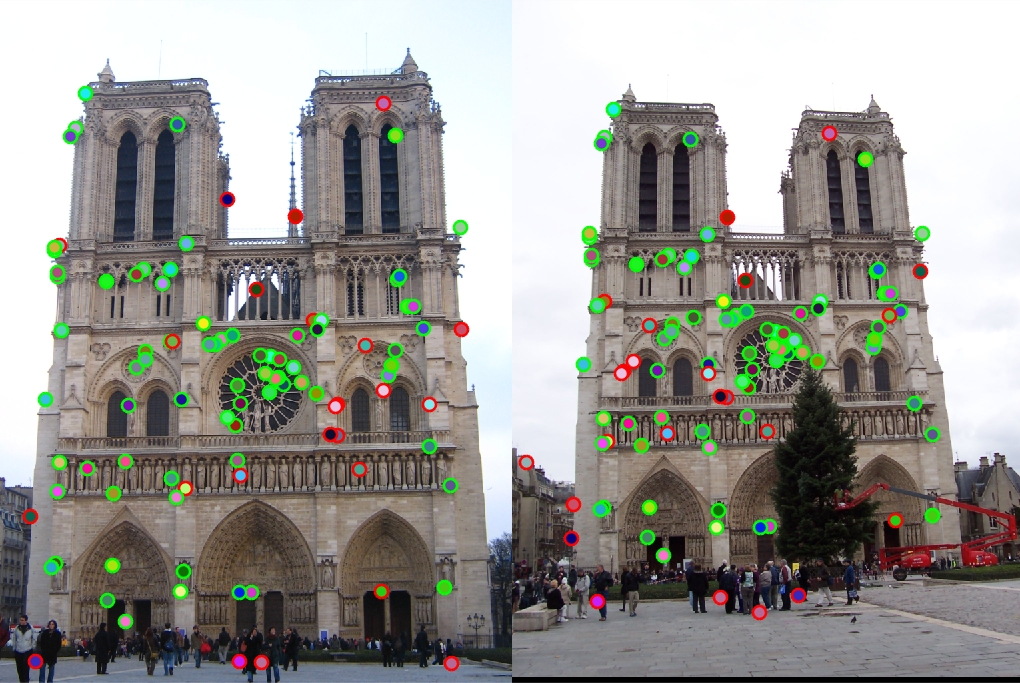
The accuracy now increases to 95% for the 100 most confident matches, a large increase over the previous iteration which did not utilize the ratio test. In order to determine the effectiveness of SIFT-like descriptors, the process was rerun using normalized patches as descriptors and the ratio test enabled.
|
The accuracy falls back down to 76%, showing that the SIFT-like features are indeed a better descriptor given that ambiguous matches are thrown out.
Additional Results
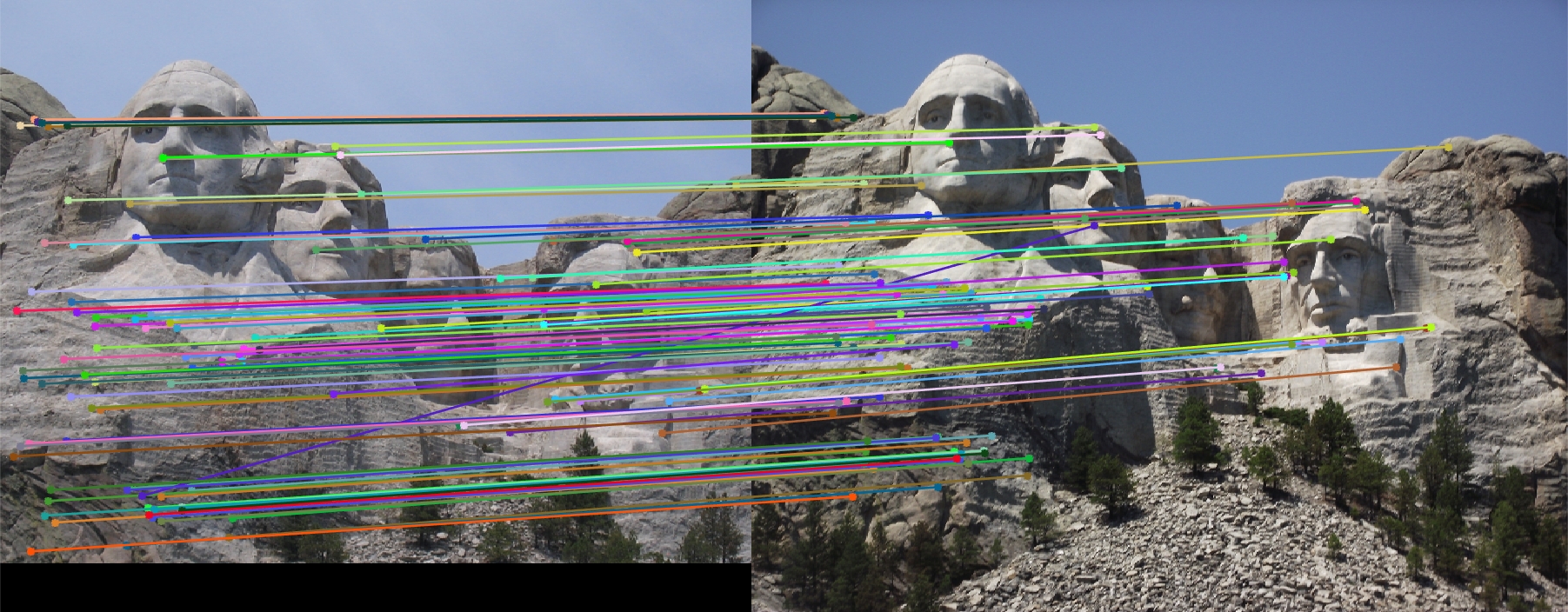
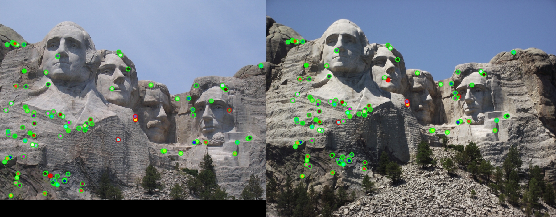
|
Working on a pair of images showing Mt. Rushmore, the program still does very well using SIFT features and the ratio test, giving a 95% accuracy for the 100 most confident matches. Given that the scale of both images is similar, using Harris corners and then SIFT-like descriptors still provides a good way to find matches.
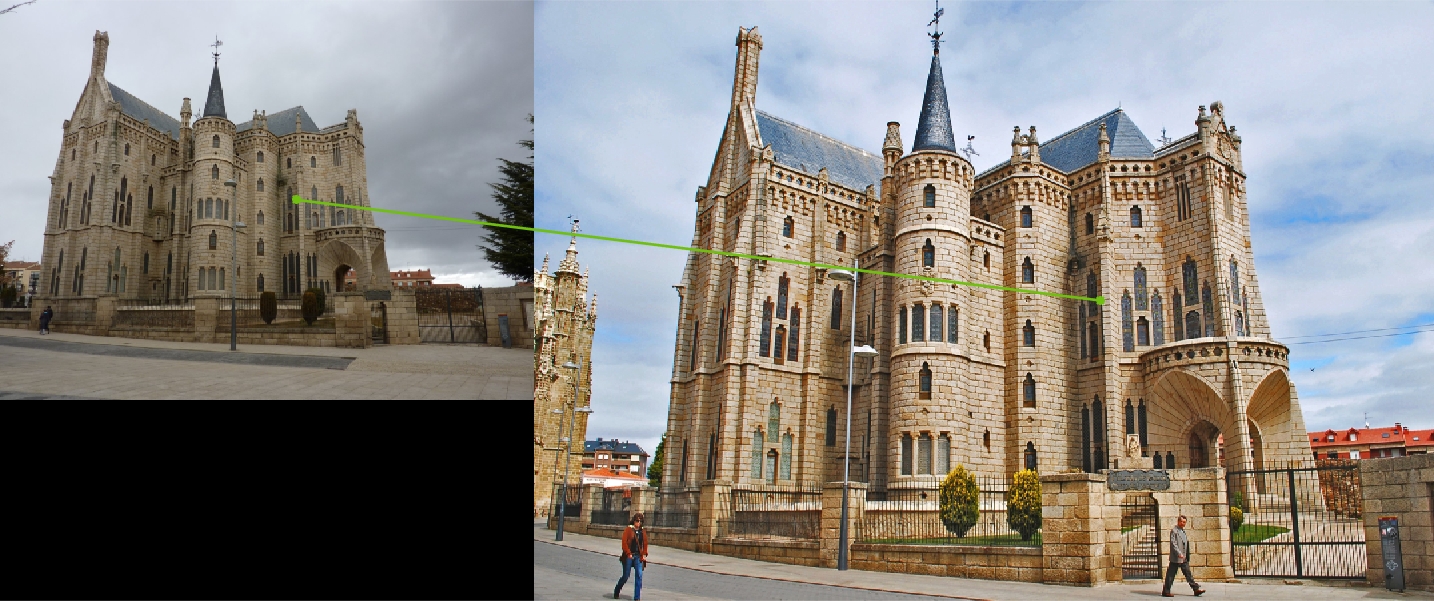
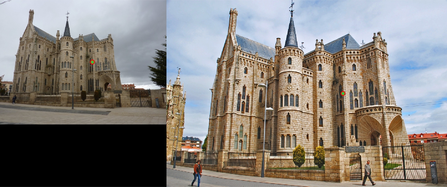
|
As seen in the Episcopal Gaudi example, this method fails when presented with two images of different scale. Even though around 1500 interest points were detected, only one match was found. A scale invariant feature must be implemented to get better matches and accuracies.