Zhen Liu (zliu327)

Project 2: Local Feature Matching

In this project, I implemented the following:

1. Interest Point Detection using Harris Detector
2. Descriptor Extraction
3. Desriptor Matching

Interest Point Detection

The image is first turned into grey-scale one if necessary. Only the pixels that are at least feature_width away from the image boundary are considered (because descriptor requires information from its neighborhood).

The interest point detection uses Harris detector. Which is, for each pixel (i,j) in the image:

$$ m(i,j) = \left[ \begin{array}{cc} (\frac{\partial I}{\partial x} (i,j))^2 & \frac{\partial I}{\partial x}(i,j) \frac{\partial I}{\partial y} (i,j) \notag \\ \frac{\partial I}{\partial x}(i,j) \frac{\partial I}{\partial y} (i,j) & \frac{\partial I}{\partial y} (i,j) \end{array} \right] $$ $$ M = w * m$$ $$ c(i,j) = det(M(i,j)) - 0.6 * (trace(M(i,j)))^2$$

,where w is a 2D filter, * is convolution operator and c(i,j) is the cornerness value at pixel (i,j)

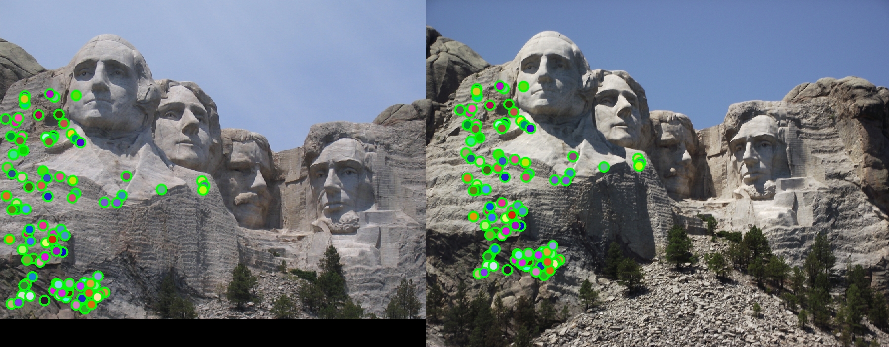
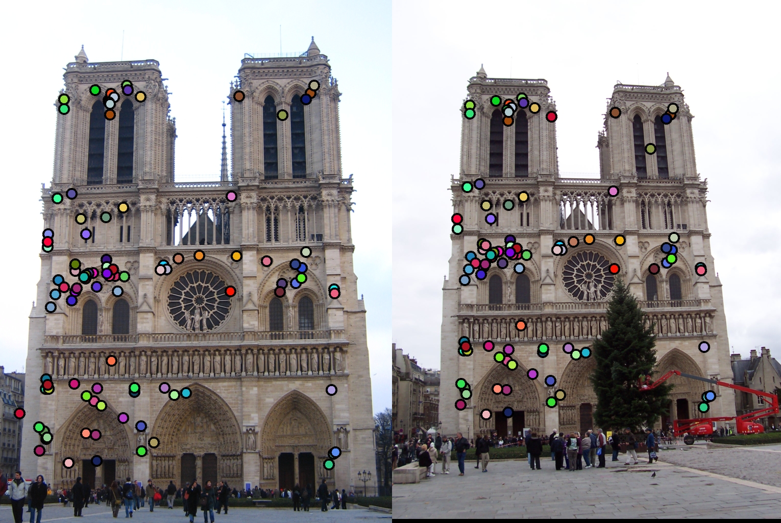
All pixels with cornerness larger than the threshold is recorded. This threshold is set to 3e-5. Non-max suppression is done by, for each connected component (every two adjacent pixels that have large enough cornerness are considered connnected), pick the weighted centroid.

At last, only the 2000 pixels with largest cornernesses are retained.

Descriptor Extraction

The descriptor is similar to SIFT. For each interest point, the (feature_width x feature_width) square region centered at interest point is used to extract information.

Before processing, the image is smoothed using Gaussian filter. Then, for each interest point, the square region is splitted into 16 subregions. At each point of each subregion, the magnitude and angle of gradient is computed. The magnitudes are smoothed using a Gaussian filter of size of the subregion.

Angles are quantized into 8 bins. Magnitudes of gradients in same angle bin are recorded, resulting in 8 values in each subregion.

For all of the 16 subregions, we have a length-128 vector by concatenating the lumped magnitude in each angle bin in each subregion calculated above (16x8=128). This vector is normalized to 1, then each dimension is clipped to 0.2. The resulted vector is normalized to 1 again, which becomes the descriptor.

Feature Matching

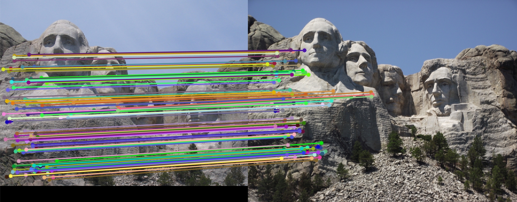
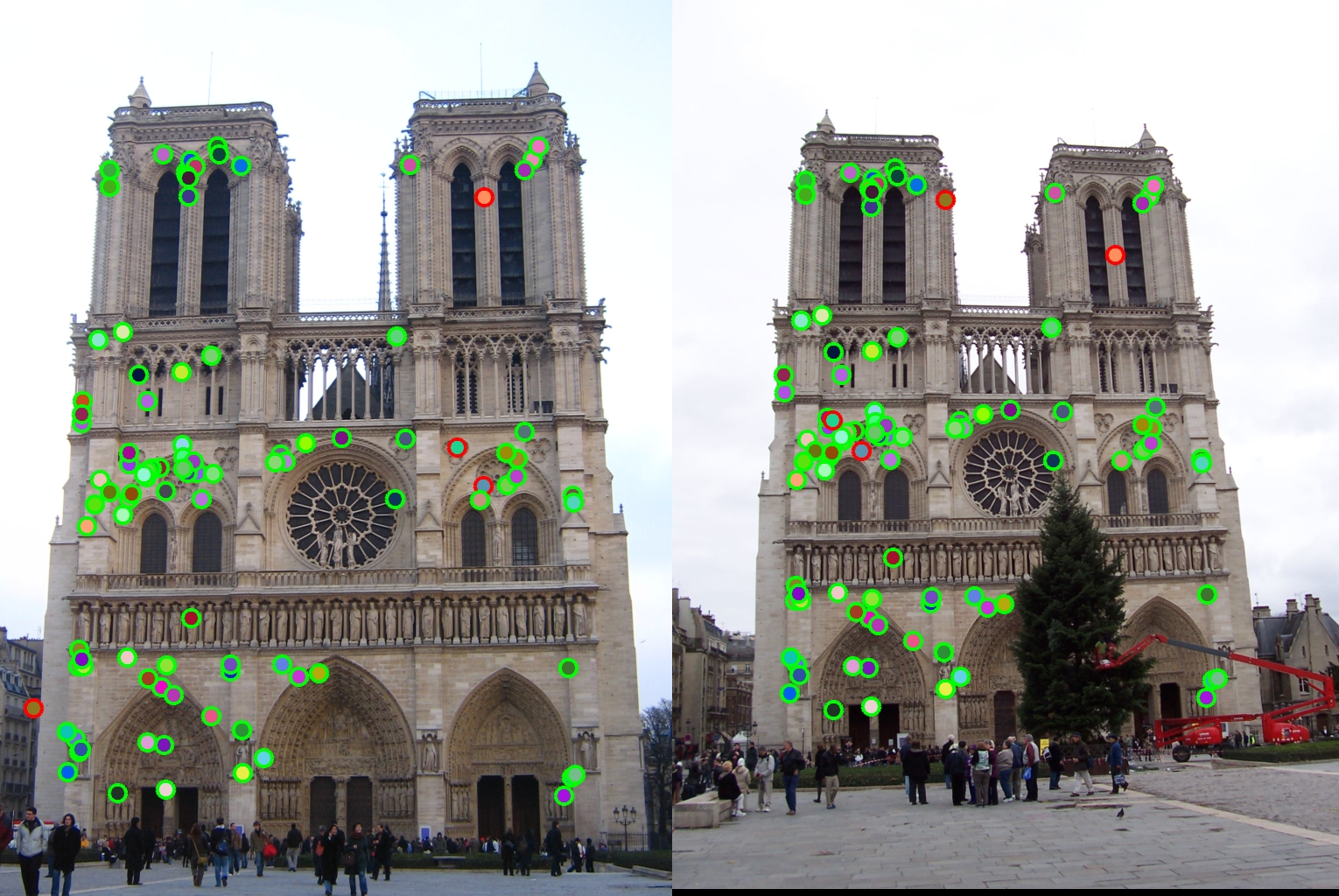
We use L2 distance to compute the fitness of pairs of features (descriptors). For each feature point in image A, we find the best and second best matching feature points in image B (using L2 distance, smaller is better). Then the ratio of best pair distance to 2nd best pair distance is computed for characterizing the confidence of each match. Then we take the best 100 matches.

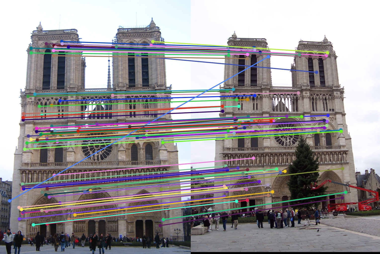
Results