Project 2: Local Feature Matching
In this project, we need to implement SIFT, a local feature matching algorithm. This algorithm includes three steps:
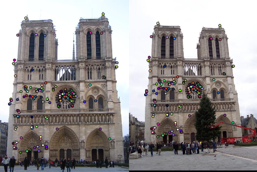
- Interest point detection.
- Local feature description.
- Feature Matching.
Algorithm
To get the interest points, we first need to compute the derivative Ix and Iy of the image. To improve the performance, I filtered them using a difference of Gaussian. Then apply a larger gaussian filter to Ix^2 and Iy^2 and IxIy. Calculate the response (det(A) - k*Trace(A)^2). Use colfilt() to do a non-maximum suppression with a threshold of 0.005 on the response.
For the local feature description, I first computed gradients of the image. Then separated them to 4 cells, calculated gradient histogram of each cell. In this project, the feature width is 16, and the number of gradient direction is 8. So we reshaped the gradient histogram to a 128 feature vector. After that, we did the normalize -> threshold -> normalize process.
To match these features, I calculate all the distance between each pair of features. Find the closest two features for each feature, compute the NNDR. If the NNDR is smaller than 0.7, the two features are matching.
Here is the core code.
% get interest points
k = 0.05;
threshold = 0.005; % 0.001 for pca
g_filter1 = fspecial('gaussian', 4) - fspecial('gaussian', 1);
g_filter2 = fspecial('gaussian', 8);
dx = [-1 0 1];
dy = dx';
Ix = conv2(image, dx, 'same');
Iy = conv2(image, dy, 'same');
Ix = imfilter(Ix, g_filter1); % to improve performance
Iy = imfilter(Iy, g_filter1);
Ix2 = conv2(Ix.^2, g_filter2, 'same');
Iy2 = conv2(Iy.^2, g_filter2, 'same');
Ixy = conv2(Ix.*Iy, g_filter2, 'same');

R = (Ix2 .* Iy2 - Ixy.^2) - k * ((Ix2 + Iy2).^2);
local_max =colfilt(R,[3,3],'sliding',@max);
[y, x] = find((R == local_max) & (R > threshold));

% get local features
feature_upper_bound = 0.6; % 0.8 for pca
g_filter = fspecial('gaussian');
image = imfilter(image, g_filter);
[grad_mag, grad_dir] = imgradient(image);
grad_mag = imfilter(grad_mag, g_filter);
grad_dir = imfilter(grad_dir, g_filter);
grad_dir = grad_dir + 180; % make all value postive

features = [];
for n = 1 : size(x)
    start_row = y(n) - feature_width / 2;
    end_row = y(n) + feature_width / 2 - 1;
    start_col = x(n) - feature_width / 2;
    end_col = x(n) + feature_width / 2 - 1;
    feature = zeros(4, 4, 8);
    if start_row >0 && start_col > 0 && end_row <= size(image, 1) && end_col <= size(image, 2)
        for i = start_row : end_row
            for j = start_col : end_col
                row = ceil((i - start_row + 1) / 4); % calculate the cell this gradient should be added to.
                col = ceil((j - start_col + 1) / 4);
                dir = mod(floor(grad_dir(i, j) / 45), 8) + 1; % take mod to make sure dir is between 1 and 8.
                feature(row, col, dir) = feature(row, col, dir) + grad_mag(i, j);
            end
        end
    end
    feature = reshape(feature, [1, 128]);
    feature = feature./norm(feature);
    feature(feature > feature_upper_bound) = 0;
    feature = feature./norm(feature);
    feature = feature.^0.5; % to improve performance, commented when using pca
    features = vertcat(features, feature);
end

% matching
num_features1 = size(features1, 1);
num_features2 = size(features2, 1);
distance = zeros(num_features1, num_features2);
matches = [];
confidences = [];

% use PCA to reduce feature dimensions.
% features1 = my_pca(features1);
% features2 = my_pca(features2);

for i = 1 : num_features1
    for j = 1 : num_features2
        distance(i, j) = sqrt(sum((features1(i, :) - features2(j, :)).^2));
    end
    sorted = sort(distance(i, :), 'ascend');
    NNDR = sorted(1)/ sorted(2);
    if NNDR < 0.7 % 0.6 for pca
        matches = vertcat(matches, [i, find(distance(i, :) == sorted(1))]);
        confidences = vertcat(confidences, 1 / NNDR);
    end
end
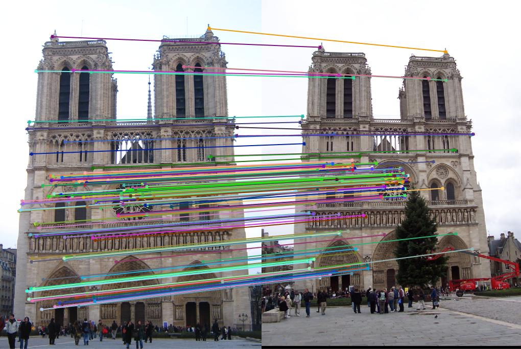
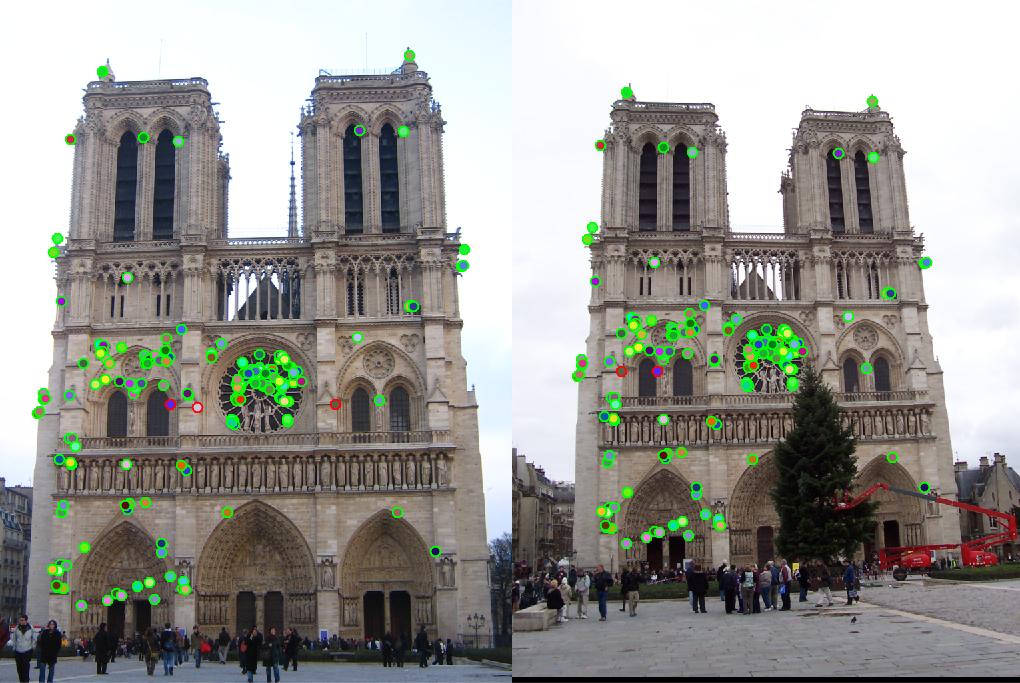
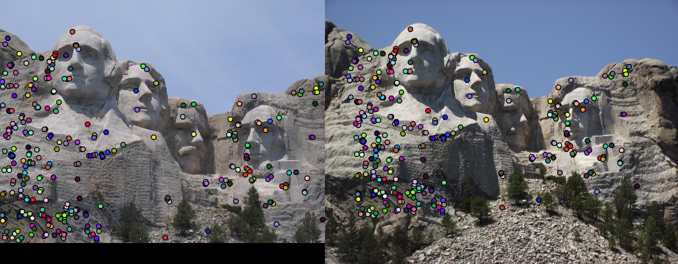
Results
|
|
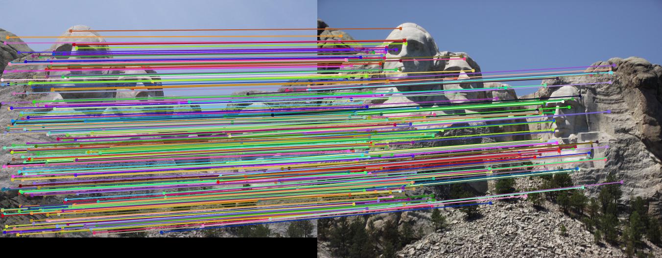
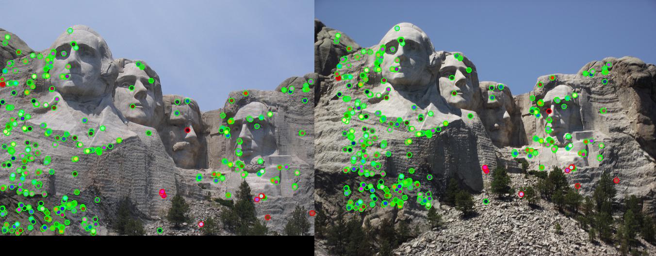
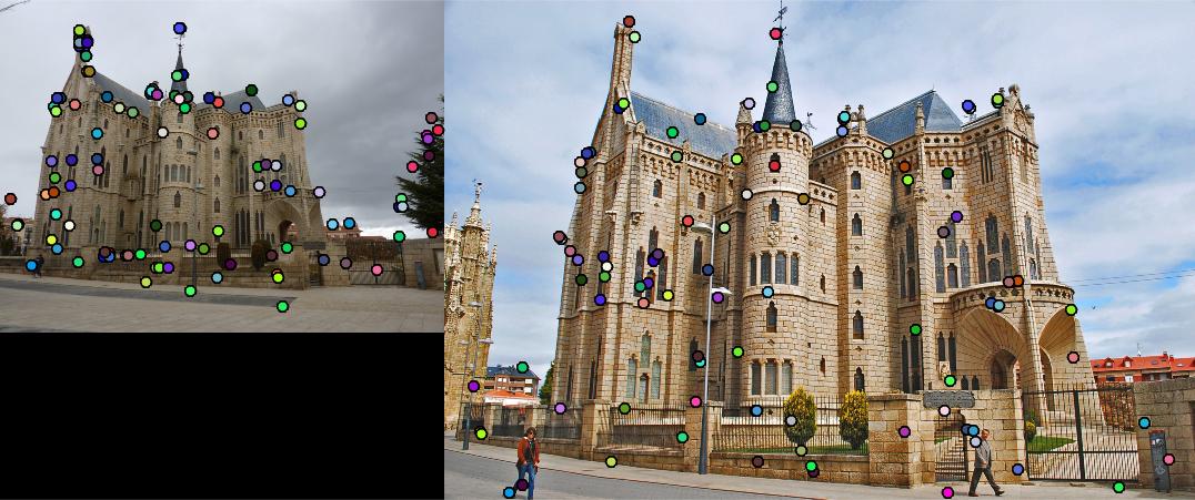
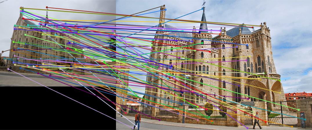
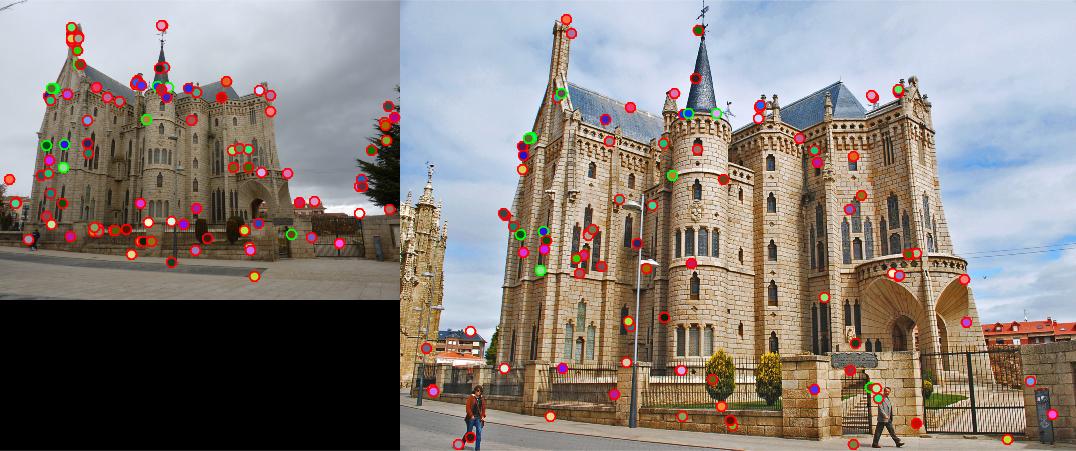
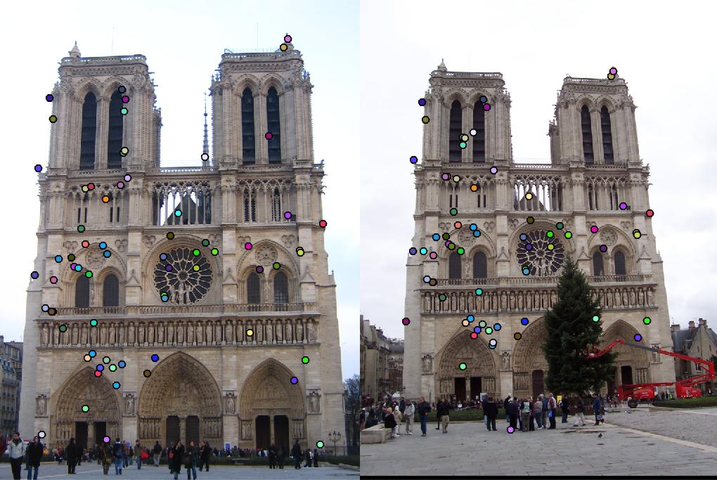
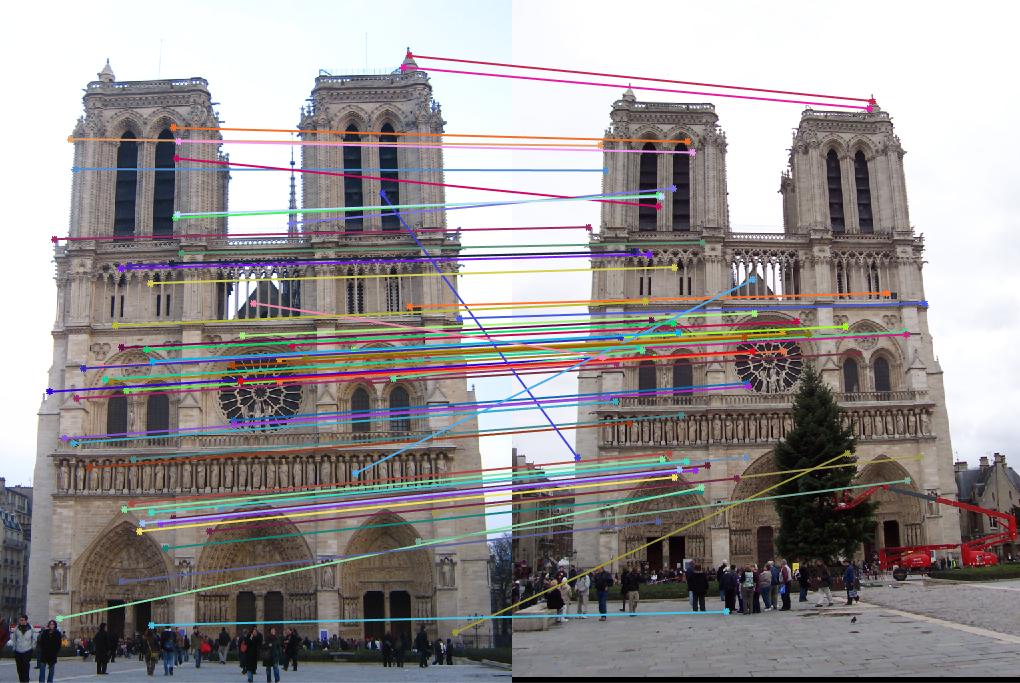
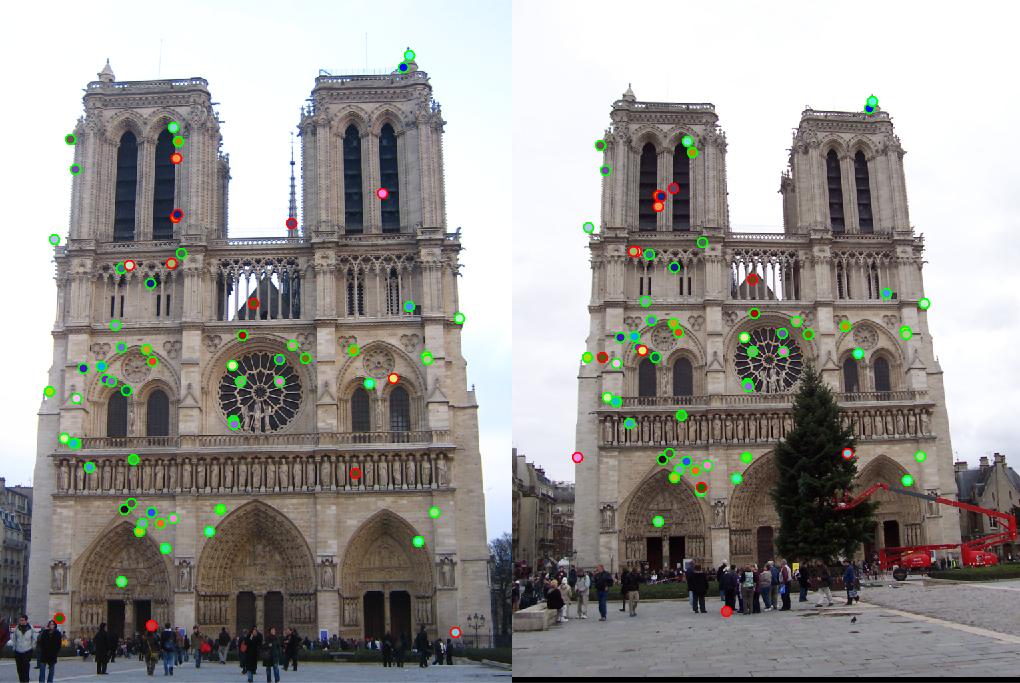
For Notre Dame, the number of good matches is 166 and the number of bad matches is 3, the accuracy is 98%. For Mount Rushmore, the number is 304/11, accuracy is 97%. These satisfy our requirements for the local feature matching. However, I failed to get matching on the third pair of images, Episcopal Gaudi. The number of features extracted from each image is 3821*128 and 30433*128, respectively, but the number of feature matched is 0. If we set the threshold for NNDR to 0.9, it could find match some features with a relative low accuracy. The result is shown as below, there are 10 good matches and 95 bad matches. The accuracy is 10%.
|
Extra credit
For extra credit, I tried to use PCA to reduce the feature dimension, from original 128 dimensions to 32 dimensions. The code is shown as below. In my_pca, I assumed the dimension of the feature is known.
	function new_features = my_pca(features)
	    num = size(features, 1);
	    new_features = [];
	    for i = 1 : num
	        coeff = pca(reshape(features(i, :), [16 8]));
	        new_feature = reshape(features(i, :), [16 8]) * coeff(:,1:2); % use only 2 basis
	        new_feature = new_feature./norm(new_feature);
	        new_features = vertcat(new_features, reshape(new_feature, [1 32]));
	    end
	end
|
To reach a acceptable accuracy, I modified some parameter to get more interest points and features. However, the final result only reached 81% accuracy. This make sense because when we use PCA to reduce the feature dimension, some feature information are lost.