Project 2: Local Feature Matching
This project explores local feature matching between images using the SIFT pipeline. Between two images of the same object the pipeline attempts to identify keypoints and match them between the two images. Three major steps are involved in the process: feature detection, feature descriptor creation, feature matching. For my implementation, a Harris corner detector with binary connected component based non-maxima suppression was used for the feature detection; a SIFT feature descriptor with 16 histogram bins of 8 directions for a total of 128 dimensions; and nearest neightbor ratio based confidence to determine the best matches.
Feature Detection
Below is my implementation of the Harris corner detector. It follows the implementation described in the slides and allows for three free parameters: alpha used in the "cornerness" function, sigma used in the Gaussian blurs, and the threshold value. The image is pre-blurred with a higher sigma than the one used on the gradients. After computing the cornerness, the threshold is used to build a binary image of the feature values and bwconncomp() is used to find the connected components. Finally, for each of the components, the maximum value is found from the original "cornerness" image and its location is used as the feature location.
alpha = 0.06;
sigma = 0.8;
threshold = 5000;
prefilter = fspecial('gaussian', feature_width, 3 * sigma);
filter = fspecial('gaussian', feature_width, sigma);
% Make the image vaues be between 0 and 255, then gaussian blur the
% original image
image = 255 * image;
image = imfilter(image, prefilter);
% Calculate the gradients for the image
[Ix, Iy] = imgradientxy(image);
% Calculate the multiplied gradients
Ix2 = Ix .* Ix;
Ixy = Ix .* Iy;
Iy2 = Iy .* Iy;
% Blur each of the multiplied gradients
gIx2 = imfilter(Ix2, filter);
gIxy = imfilter(Ixy, filter);
gIy2 = imfilter(Iy2, filter);
% Calculate the cornerness based on the formula given in the slides
har = gIx2 .* gIy2 - (gIxy .* gIxy) - alpha * ((gIx2 + gIy2) .* (gIx2 + gIy2));
% Perform non-maxima suppression to get a single point for each feature
% Threshold the values to create a binary image
harBin = har;
harBin(harBin < threshold) = 0;
harBin(harBin >= threshold) = 1;
% Using the binary image, calculate the connected components
connectedComponents = bwconncomp(harBin);
% Take the max of each connected component to find the correct value
% Only use the value though if it's not too close to the edge
x = [];
y = [];
for i=1:connectedComponents.NumObjects
	connectedComponent = connectedComponents.PixelIdxList{i};
	maxPixelIndex = connectedComponent(1);
	maxPixelValue = har(maxPixelIndex);
	for j=2:size(connectedComponent)
		currentIndex = connectedComponent(j);
		currentValue = har(currentIndex);
		if currentValue > maxPixelValue
			maxPixelIndex = currentIndex;
		end
	end
	[iY, iX] = ind2sub(size(har), maxPixelIndex);
	if iX > feature_width / 2 && iX < size(image, 1) - feature_width / 2 ...
	  && iY > feature_width / 2 && iY < size(image, 2) - feature_width / 2
		x = [x; iX];
		y = [y; iY];
	end
end
Feature Descriptor Creation
Below is my implementation of the SIFT feature descriptor. It uses imgradientxy() to get the gradients as it works well and doesn't take too much time. While looping through each of the features, it picks which histogram bin to add the gradient magnitude based on the cell the pixel is in and the angle of the gradient vector. I found that this gave pretty good descriptors without the interpolation described in the original algorithm. In order to get slightly more robust features, the normalize -> threshold -> normalize operation is performed like in the original implementation. This tended to give me slightly better results for very little time cost.
% Take the image gradients and pad just in case any near-edge features
% slipped through to prevent errors being thrown
[gx, gy] = imgradientxy(image);
padding = feature_width / 2;
gx = padarray(gx, [padding padding]);
gy = padarray(gy, [padding padding]);
% Loop through each feature and calculate its descriptor
features = zeros(size(x, 1), 128);
for f = 1:size(features, 1)
    % Get the current features feature_width x feature_width gradient cell
    curX = int32(x(f));
    curY = int32(y(f));
    currentXGradients = gx(curY:curY + feature_width - 1, curX:curX + feature_width - 1);
    currentYGradients = gy(curY:curY + feature_width - 1, curX:curX + feature_width - 1);
    for r = 1:feature_width
        for c = 1:feature_width
            % For each pixel in the feature cell, calculate what desciptor
            % cell it falls in, then the bin based on the gradient
            % direction
            cellX = floor((c - 1) / 4);
            cellY = floor((r - 1) / 4);
            xGrad = currentXGradients(r, c);
            yGrad = currentYGradients(r, c);
            gradDir = atan2(yGrad, xGrad);
            if gradDir <= pi / 8 && gradDir >= -pi / 8
                gradDir = 1;
            elseif gradDir > pi / 8 && gradDir <= 3 * pi / 8
                gradDir = 2;
            elseif gradDir > 3 * pi / 8 && gradDir <= 5 * pi / 8
                gradDir = 3;
            elseif gradDir > 5 * pi / 8 && gradDir <= 7 * pi / 8
                gradDir = 4;
            elseif gradDir < pi / 8 && gradDir >= -3 * pi / 8
                gradDir = 8;
            elseif gradDir < -3 * pi / 8 && gradDir >= -5 * pi / 8
                gradDir = 7;
            elseif gradDir < -5 * pi / 8 && gradDir >= -7 * pi / 8
                gradDir = 6;
            else
                gradDir = 5;
            end
            features_index = gradDir + 8 * cellX + 32 * cellY;
            % Take the magnitude and add it to the bin it should go in
            gradMag = norm([xGrad yGrad]);
            features(f, features_index) = features(f, features_index) + gradMag;
        end
    end
    % Normalize the feature vectors for each histogram cell
    for cell = 1:16
        features(f, 1 + (cell - 1) * 8:8 + (cell - 1) * 8) = features(f, 1 + (cell - 1) * 8:8 + ...
          (cell - 1) * 8) / norm(features(f, 1 + (cell - 1) * 8:8 + (cell - 1) * 8), 2);
    end
    % Cap out any value at 0.2
    for i = 1:128
        if features(f, i) > 0.2
            features(f, i) = 0.2;
        end
    end
    % Renormalize the vectors
    for cell = 1:16
        features(f, 1 + (cell - 1) * 8:8 + (cell - 1) * 8) = features(f, 1 + (cell - 1) * 8:8 + ...
          (cell - 1) * 8) / norm(features(f, 1 + (cell - 1) * 8:8 + (cell - 1) * 8), 2);
    end
end
Feature Matching
Below is my implementation of the feature matching. It uses the nearest neighbor distance ratio to determine the confidence that each feature matches. To achieve this, it just loops through the image with fewer features and matches the best feature from the other image. This means that each final feature in the image is mapped to a unique feature in the other image. This affected accuracy slightly, but I thought gave much nicer final results in that multiple features in one image could not map to a single feature in the other image. All of the distances are precomputed and stored in the distances matrix, and calculating these distances was by far the longest portion of my algorithm.
% Set up the confidence, matches, and distances arrays
num_features = min(size(features1, 1), size(features2,1));
matches = zeros(num_features, 2);
confidences = zeros(num_features,1);
matchedOtherIndices = zeros(num_features, 1);
distances = zeros(size(features1, 1), size(features2, 1));
% Precompute the Euclidian distance for all desciptors
for f1 = 1:size(features1, 1)
    for f2 = 1:size(features2, 1)
        distances(f1, f2) = pdist2(features1(f1,:), features2(f2,:));
    end
end
if size(features1, 1) < size(features2, 1)
    % Loop through all of the features in features1 as the originating
    % feature
    for f1 = 1:size(features1,1)
        % Find the best and second best match based on the distance between
        % the two features
        bestMatchIndex = -1;
        bestMatchDistance = 0;
        secondMatchIndex = -1;
        secondMatchDistance = 0;
        for f2 = 1:size(features2,1)
            dist = distances(f1, f2);
            if (bestMatchIndex == -1 || dist < bestMatchDistance) && ~ismember(f2, matchedOtherIndices)
                bestMatchIndex = f2;
                bestMatchDistance = dist;
            end
        end
        for f2 = 1:size(features2,1)
            dist = distances(f1, f2);
            if ((secondMatchIndex == -1 || dist < secondMatchDistance) && f2 ~= bestMatchIndex)
                secondMatchIndex = f2;
                secondMatchDistance = dist;
            end
        end
        % Calcuate the nearest neighbor distance ratio based on the first
        % and second nearest neighbor
        ratio = bestMatchDistance / secondMatchDistance;
        matches(f1, 1) = f1;
        matches(f1, 2) = bestMatchIndex;
        confidences(f1) = 1 / ratio;
        % Add the selected index to a list of selected indices so that we
        % don't end up finding matches between the same features
        matchedOtherIndices(f1) = f2;
    end
else
    % Loop through all of the features in features1 as the originating
    % feature
    for f2 = 1:size(features2,1)
        % Find the best and second best match based on the distance between
        % the two features
        bestMatchIndex = -1;
        bestMatchDistance = 0;
        secondMatchIndex = -1;
        secondMatchDistance = 0;
        for f1 = 1:size(features1,1)
            dist = distances(f1, f2);
            if (bestMatchIndex == -1 || dist < bestMatchDistance) && ~ismember(f1, matchedOtherIndices)
                bestMatchIndex = f1;
                bestMatchDistance = dist;
            end
        end
        for f1 = 1:size(features2,1)
            dist = distances(f1, f2);
            if ((secondMatchIndex == -1 || dist < secondMatchDistance) && f1 ~= bestMatchIndex)
                secondMatchIndex = f1;
                secondMatchDistance = dist;
            end
        end
        % Calcuate the nearest neighbor distance ratio based on the first
        % and second nearest neighbor
        ratio = bestMatchDistance / secondMatchDistance;
        matches(f2, 1) = bestMatchIndex;
        matches(f2, 2) = f2;
        confidences(f2) = 1 / ratio;
        % Add the selected index to a list of selected indices so that we
        % don't end up finding matches between the same features
        matchedOtherIndices(f2) = f1;
    end
end
Feature Matching Results
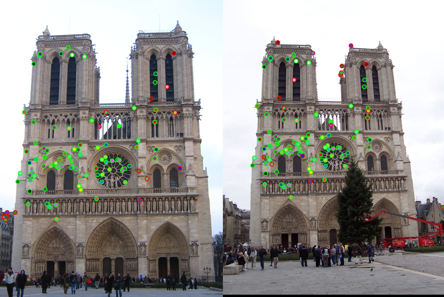
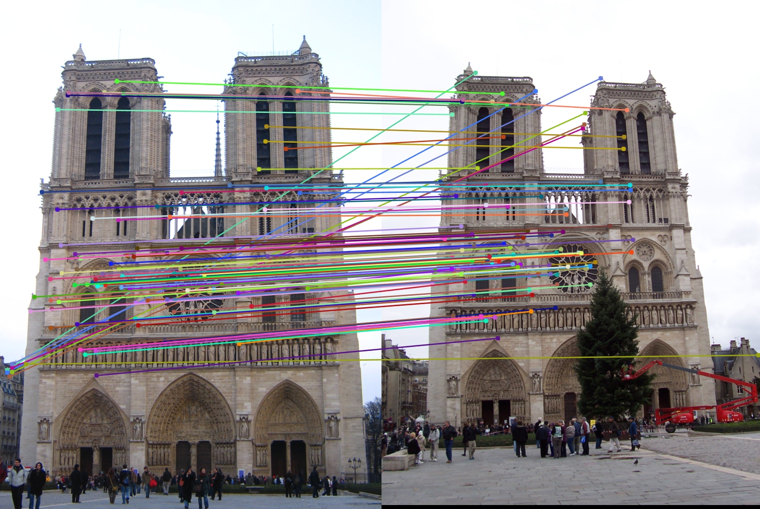
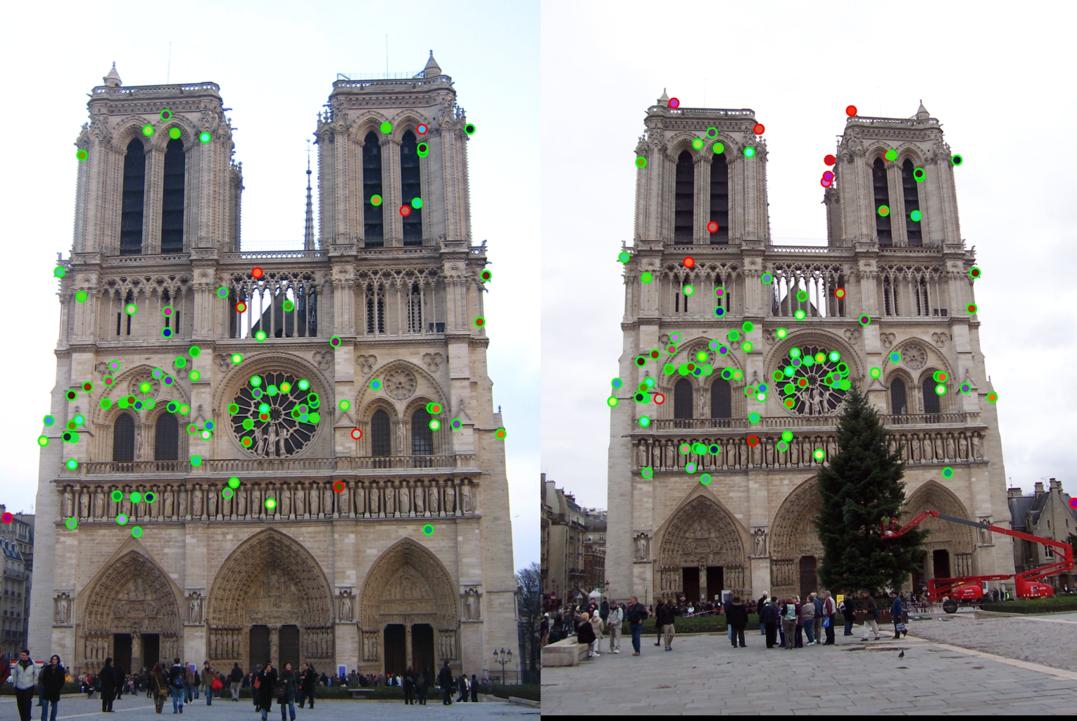
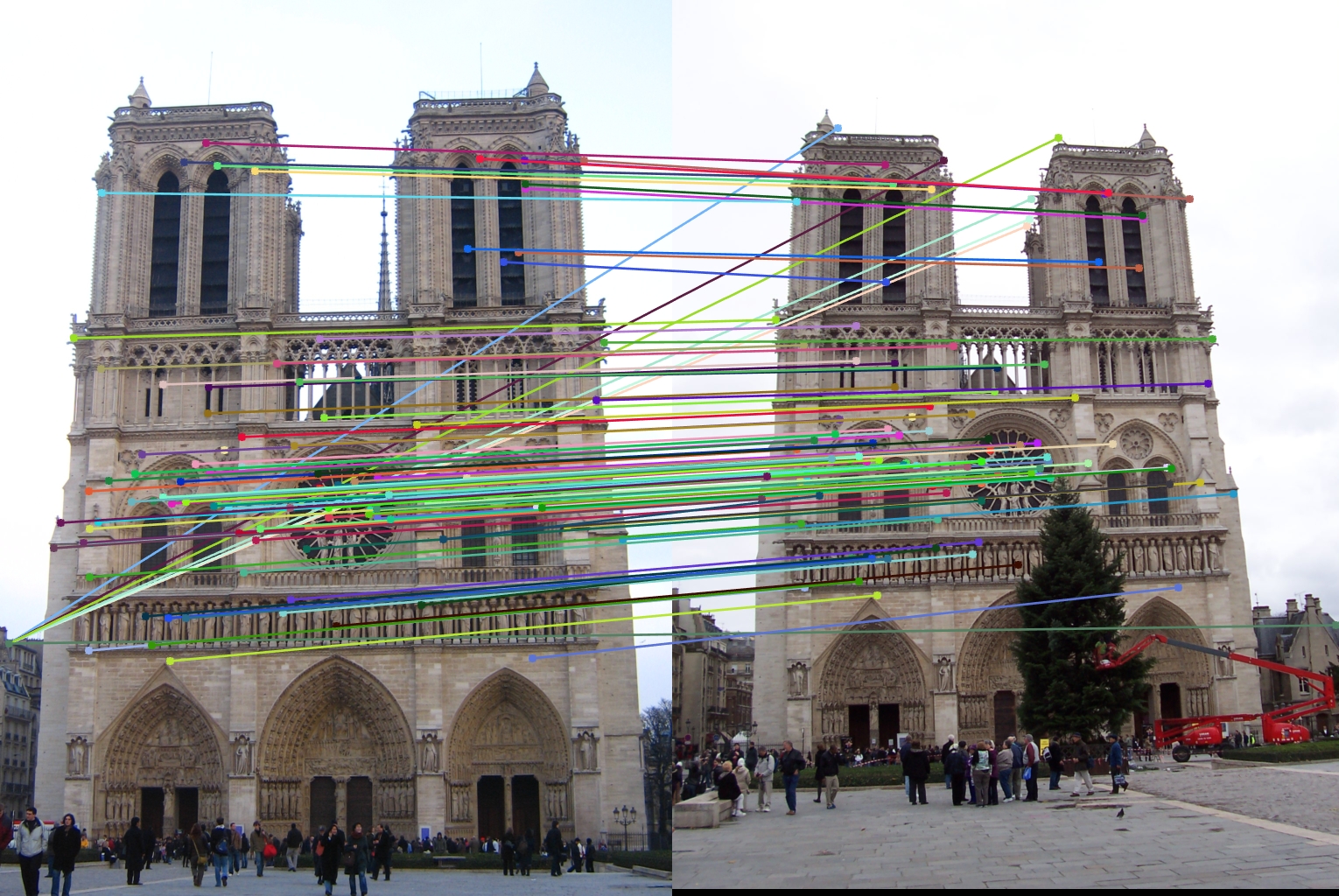
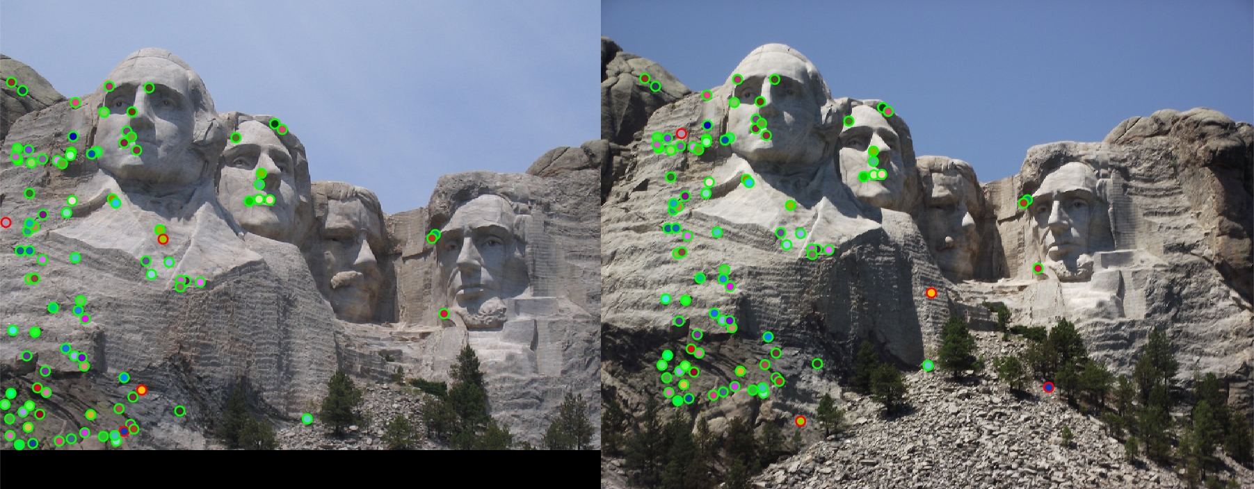
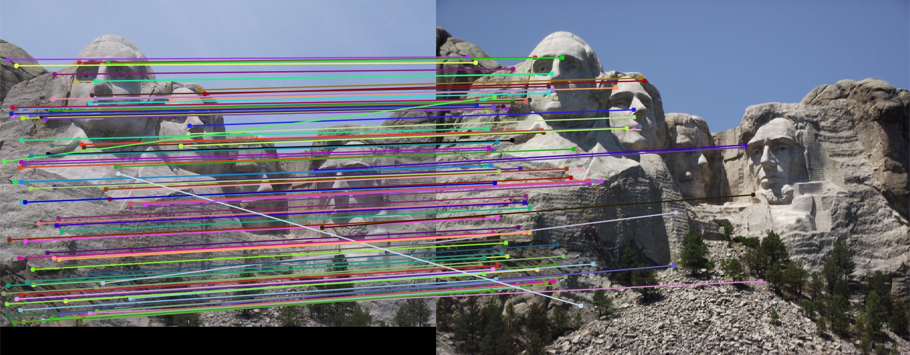
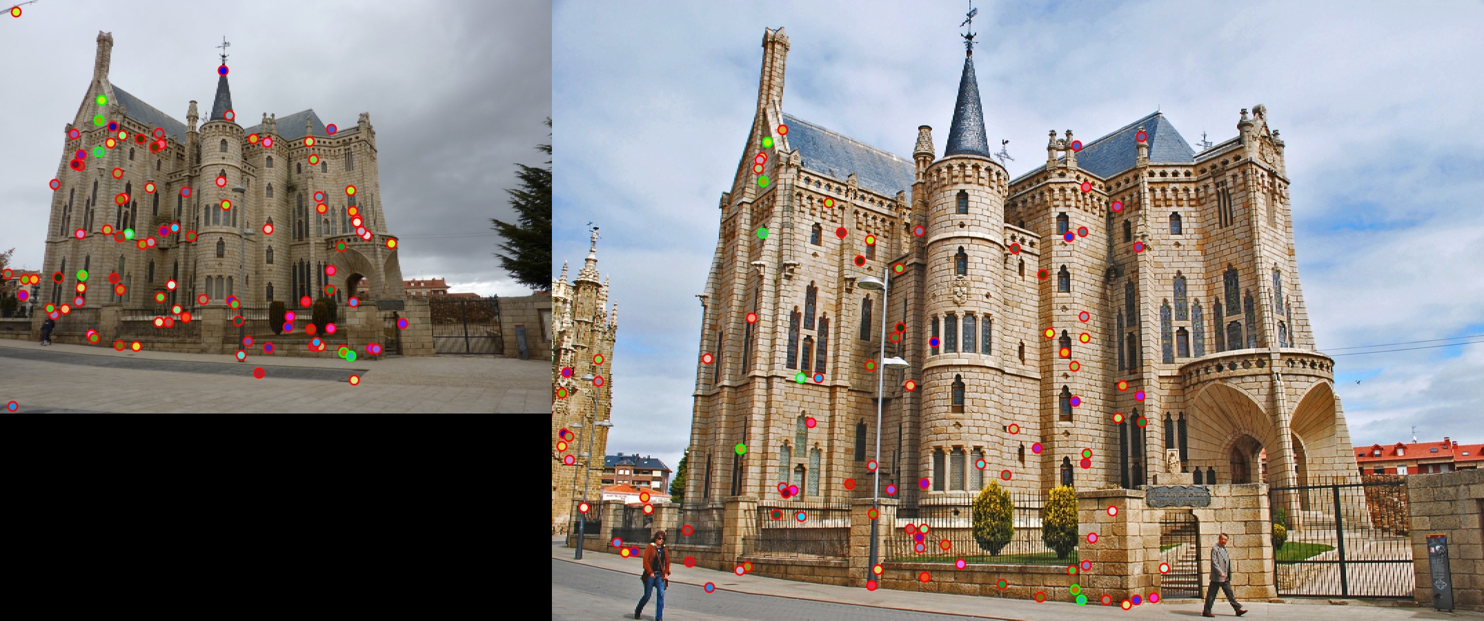
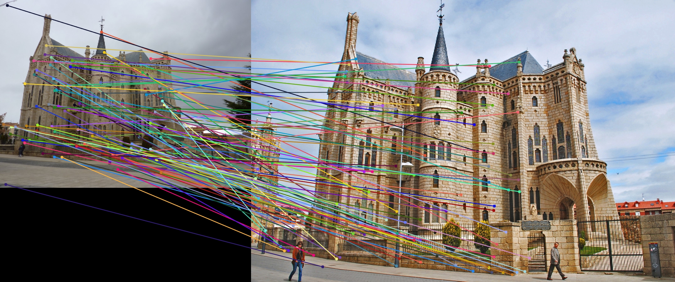
The feature matching pipeline was run on three different sets of input images: Notre Dame, Mount Rushmore, and Episcopal Guadi. Both Notre Dame and Mount Rushmore provided very good results, with Notre Dame making 83% accuracy and Mount Rushmore surprisingly having a better accuracy of 96%. This could have been a result of the corner detector producing more distinct feature points, as the church tends to have longer beams that are harder to look at, or the SIFT descriptors being more unique for Mount Rushmore, again since it doesn't have the support beams of the cathedral or the repeating architectural features. This could also have simply been the result of a lucky tuning with the parameters though. The Episcopal Gaudi faired much worse, only getting about 5% accuracy. The two images were quite a bit different from each other though and my descriptors did not have any support for scale or rotation invariance, which is most likely to blame. Notre Dame was run with duplicates allowed and duplicates not allowed, and the duplicates can be seen in the middle left of the left image.
The following images show the results of my implementation. In order they are:
- Notre Dame with duplicates not allowed - 83% accuracy
- Notre Dame with duplicates allowed - 87% accuracy
- Mount Rushmore - 96% accuracy
- Episcopal Gaudi - 7% accuracy
|
|
|
|